Weasis provides the tools to visualize and analyze images obtained from medical imaging equipment according to the DICOM standard. This free DICOM viewer is used by healthcare professionals, researchers and patients.
If you are new to Weasis, it is recommended to read this page to understand the main elements of the interface.
The tutorials are organized by topics and can be read independently.
If you find any errors or inaccuracies, just click the Edit button displayed on top right of each page, and make a pull request to submit your changes.
Subsections of Tutorials
GUI Overview
Essential aspects of the interface
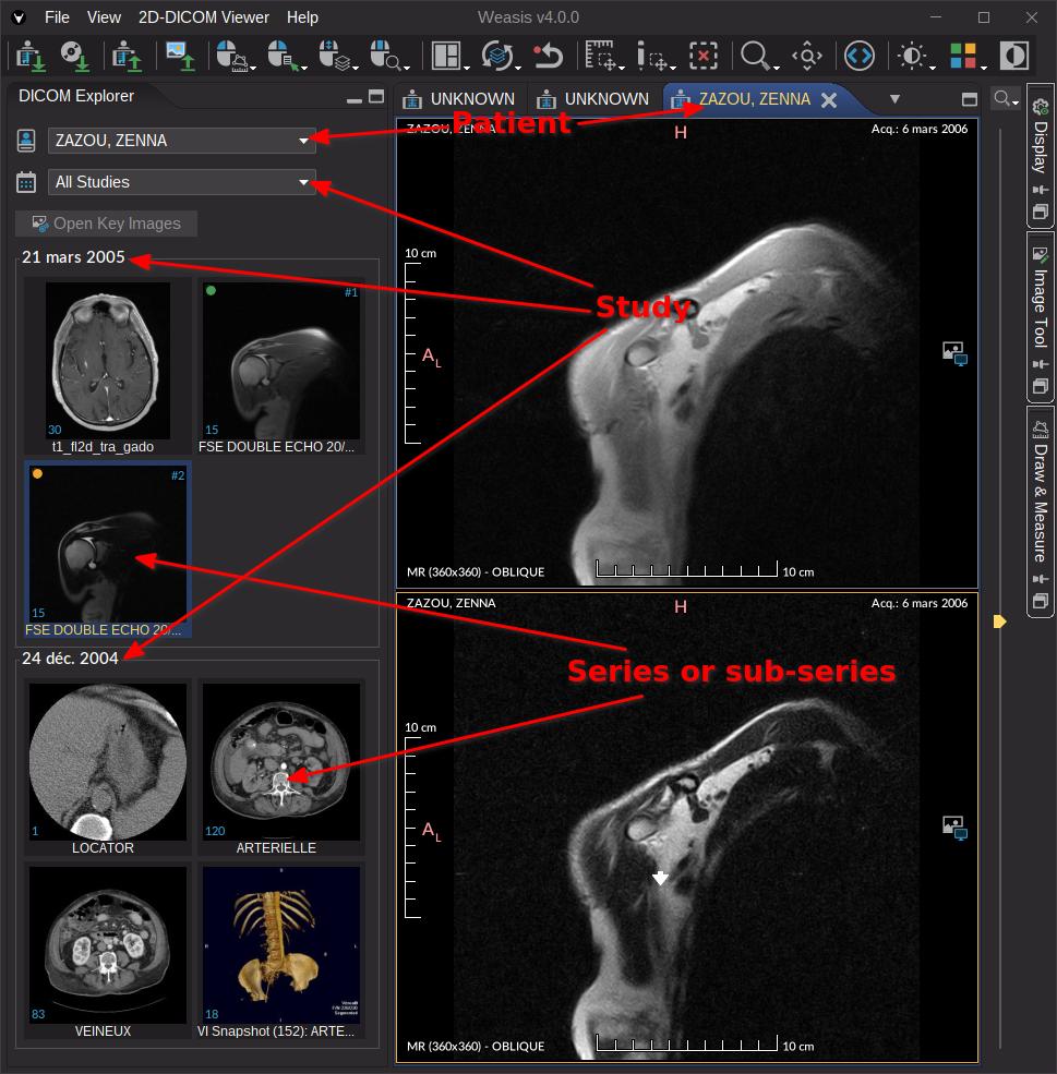
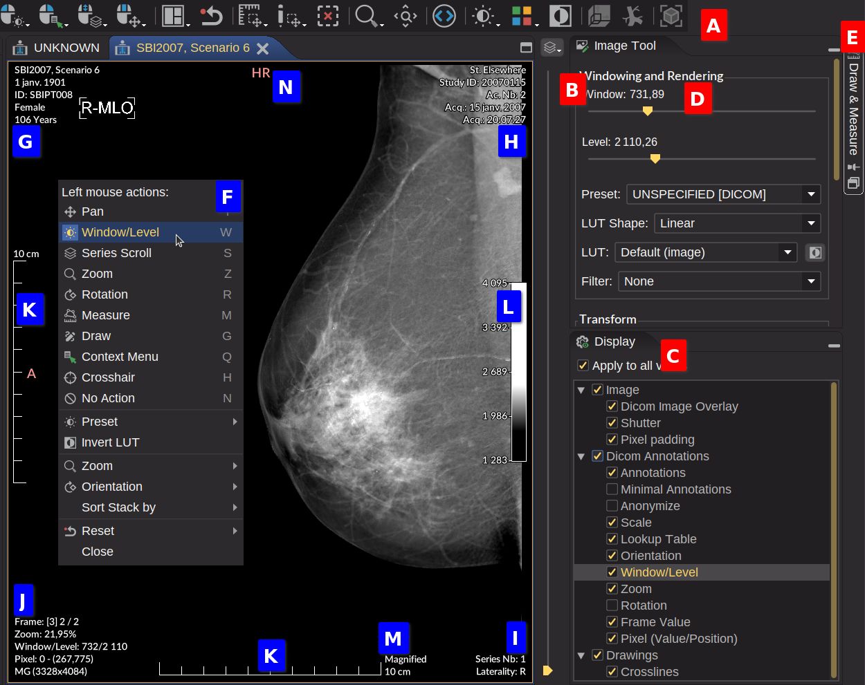
The following image shows the main elements of the graphical user interface (GUI). For more detailed documentation on the various elements of the interface, click on the green or blue areas of the image.
The interface of the default DICOM workspace consists mainly of 2 parts:
The DICOM Explorer on the left (in blue). It allows you to import and export data, as well as select the series to be visualized.
Depending on the data imported, different viewer/player types (represented by a tab) are displayed in the main section (green). Menus , toolbars and tools change according to the type of viewer selected.
The selected viewer is the image above is the DICOM 2D viewer
which is the viewer opened by default.
A tab containing a multi-view layout can display images from only one patient. However, one patient can appear in several tabs.
A tab is also docked panel that can be arranged by dragging and dropping it to the desired location. This makes it possible to display 2 tabs side by side.
See also DICOM Explorer to understand how to navigate through the Patient/Study/Series/Image.
Note
Select your preferred language and regional settings in the preferences. Adapt the graphical interface to your needs by modifying the theme or the scaling factor for a better user experience on HiDPI screens.
Tip
In the View menu at the top, toolbars and tools related to the selected viewer can be shown or hidden. These display preferences are retained even after a restart. Only Explorer preferences are retained for the duration of the session.
List of other viewers/Players in the DICOM workspace
DICOM PDF viewer (default system application associated with pdf files). Same for other encapsulated documents.
DICOM Video player (default system player associated with mpg files)
List of other workspaces
Dicomizer
Explorer of standard images (based on the non-dicom-explorer.json configuration profile)
DICOM Import
How to import DICOM files
Weasis can open DICOM files from various ways and sources: drag and drop, local device, DICOM ZIP, DICOM CD/DVD, DICOM Query/Retrieve, and from commands locally or remotely.
Note
An popup error message is displayed when DICOM files cannot be read (from v4.3.0) or when a network error occurs. In the latter case a message asking to download again the missing files.
From the system file explorer
Drag and drop
Files or folders selected from the system file explorer can be opened by dragging and dropping into the central area of Weasis.
Empty central panel: Any files than ca be open by one of the viewers (e.g. standard images such as TIFF, PNG, JPEG…)
DICOM Explorer and DICOM viewers (SR, AU, MPR, 2D and 3D) in the central panel: Only DICOM files. Opens the default viewer according to the files.
File association
Dicom files can be opened by double-clicking them from the system file explorer.
Note
On Windows only the files with the extension “.dcm” are associated with Weasis. With other systems DICOM without extension are associated with Weasis.
From Weasis menu or toolbar
From the main menu, open File > Import > DICOM or from the first import button in the toolbar.
In order to import DICOM CD/DVD go the main menu, open File > Import > DICOM CD or from the second import button in the toolbar.
Local Device
Files and/or folders: list of selected items or unique path
Search recursively: when this option is activated the import takes into account the subdirectories
Open in new tab: behavior to automatically open the images of a patient when loading DICOM files
DICOM ZIP
Select: browse a DICOM zip file. When the archive file is encrypted, a password prompt is displayed.
Open in new tab: behavior to automatically open the images of a patient when loading DICOM files
DICOMDIR
It may be from a DICOM CD/DVD or a folder containing a DICOMDIR
Path: browse a folder containing a DICOMDIR
Detect CD-ROM: try to load a DICOM CD/DVD
Copy images into the local temporary directory: useful for slow reading device like CD-ROM
DICOM Query/Retrieve
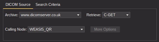
On DICOM Source tab:
Archive: select the archive to query
With DICOM nodes: classic DIMSE C-Find with C-Move, C-Get or WADO-URI for retrieving DICOM files
With DICOMWeb nodes: QIDO and WADO-RS for retrieving DICOM files (no other options are required)
Retrieve (only with DICOM archive): the protocol to retrieve the images
C-MOVE: the classic DIMSE protocol (accepts all sop classes, not recommended for WEB)
C-GET: transfer syntaxes are negotiated by each sop classes according to a configuration file
WADO-URI: required a WADO server (C-Find + WADO retrieve)
Calling Node (only with DICOM archive): select the adapted calling DICOM node
More options: allows you to open the preferences to configure the DICOM nodes
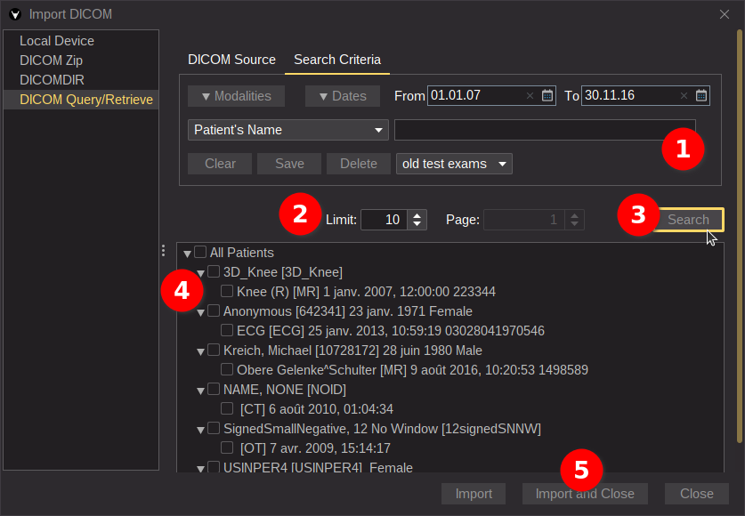
On Search Criteria tab:
Select a pre-registered item (bottom right of the Search Criteria panel) or Fill the search criteria. Criteria can be saved and reuse later, since Version4.1.0 the item selected in the combo box is automatically applied the next time this window is opened (the default value is Empty).
Adjust the limit to the maximum number of exams in the response. Set the limit to 0 to avoid this constraint. For DICOMWeb the limit is the number of elements on a page, and you can go to the next page with the spinner buttons.
Click on Search
Select the exams you want to import
Start importing and close the window
Note
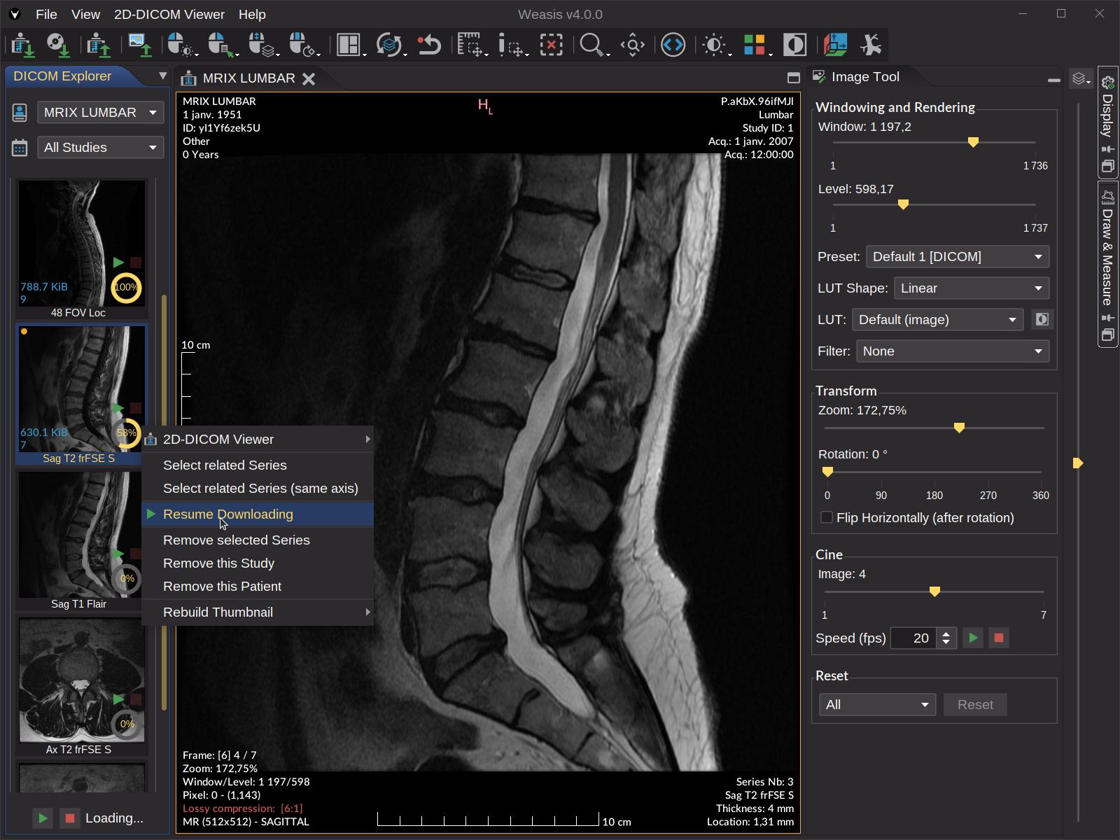
The progression of downloaded images for a series and the ability to pause the download of a series is only possible with DICOMWeb nodes and with the combination (DICOM C-FIND + WADO-URI).
Resuming the download of a series by clicking on the green play button or from the contextual menu.
Tip
When a query is too long, try to click on the Clear button in Search Criteria in order to cancel the request.
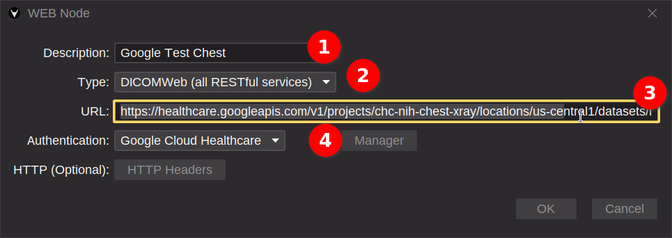
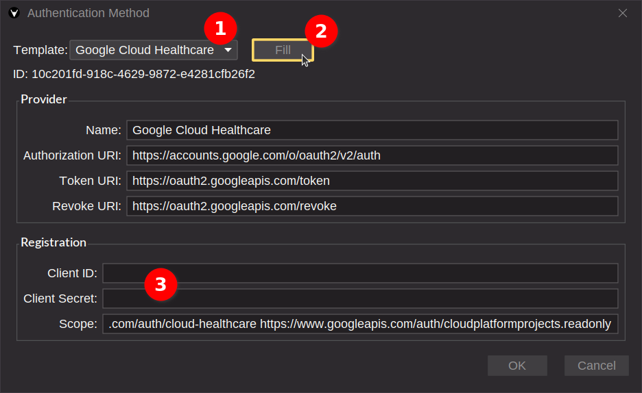
With a DICOMWeb node, a login from a web browser can be required (e.g. login to your Google account). If something goes wrong Weasis may freeze for at least 1 minute waiting for the authorization code.
This page explains how to configure a remote archive in DICOMWeb and then use this DICOMWeb node to retrieve exams remotely. However, it is also possible, without any prior configuration, to launch Weasis from a web context by passing it some parameters to retrieve images in DICOMWeb.
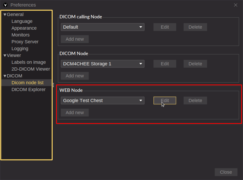
From the main menu, open File > Preferences (Alt + P) and select DICOM node list.
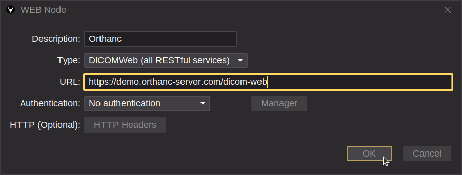
Currently, the DICOMWeb service of Orthanc doesn’t support the thumbnail service.
Create a new DICOMWeb node with the following URL (example with the demo server without authentication):
https://demo.orthanc-server.com/dicom-web
dcm4chee-arc-light
Kheops
DICOM Export
How to export DICOM files
Exporting the selected view
From the toolbar icon
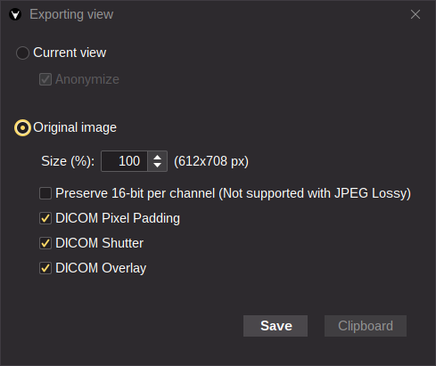
or from the main menu File > Export > Exporting view export the selected view either to the clipboard or to image file (PNG, TIF, JPG, JPEG2000).
Current view
Export the view as it is (size and overlay).
Anonymize: It allows you to remove identifying information in overlay.
Original Image
Export the view according to the original image with some options.
Size: Change the image size in percent
Preserve 16-bit per channel: Option to preserve the pixel depth (e.g. 16-bit in PNG/JPEG 2000/TIFF, double values in TIFF). When this option is applied, the pixel values will match with the Modality LUT values (e.g. Hounsfield values). Exporting in JPEG Lossy is only possible when unchecked for 8-bit image.
In order to open the DICOM export window click on toolbar icon
or from the main menu File > Export > DICOM
Local Device
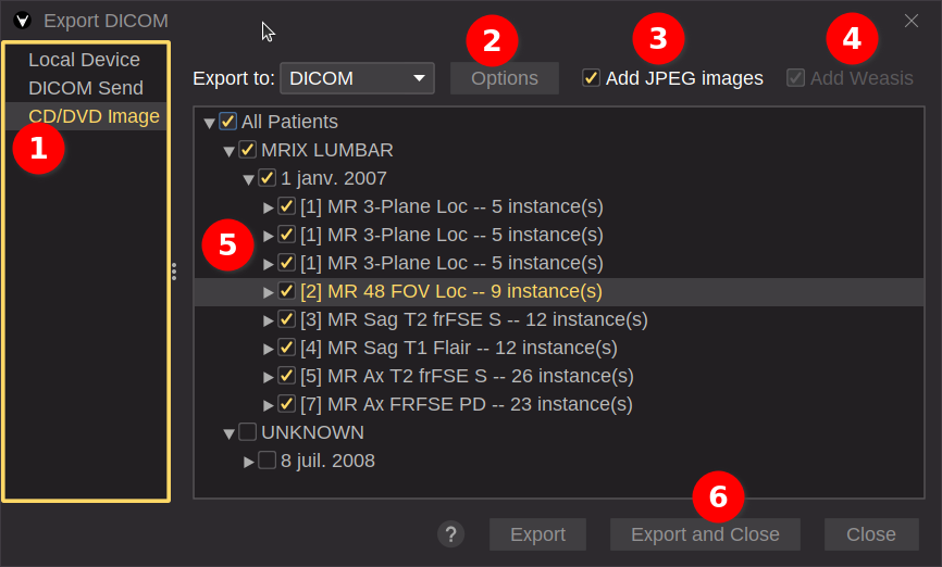
Select Local Device item
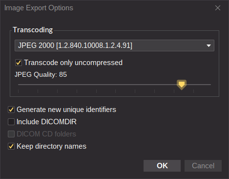
Choose the exporting options
Transcoding: It allows you to change the DICOM transfer syntax. Use this option only if you understand well what you are doing.
Generate new unique identifiers: Create new UIDs for some attributes. Within an export, the consistency between all the UIDs and their references is preserved.
Include DICOMDIR: Create DICOMDIR file
DICOM CD folders: Add a directory to be compliant with DICOM CD
Keep directory names: Preserve the name in the directory hierarchy (not compliant with DICOMDIR)
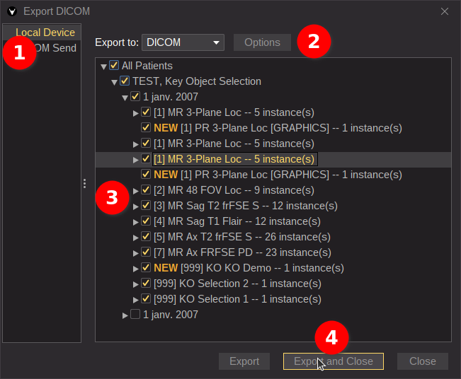
Select the patient/study/series/instance to export. Note: series created by Weasis have a flag “NEW”
Export the selection and close the Window
Tip
When opening the Export DICOM window, the checkbox of the study selected in the viewer (surrounded by an orange line) is automatically checked and open series have a full-line selection.
In order to help with series selection, place the cursor on a series line, and you’ll see a tooltip displaying its thumbnail.
Note
When DICOM data is exported in a native image format (JPG, PNG, JPEG 2000 or TIFF), only the images are transformed (see original image options) and the encapsulated files (video, audio and PDF) are extracted.
Multiframe images are exported by adding a number to the end of the file name.
DICOM Send
Select DICOM Send item
Select the destination node (either a DICOM node or a DICOMWeb node)
Select the patient/study/series/instance to export. Note: series created by Weasis have a flag “NEW”
Send the selection to the destination and close the Window
CD/DVD Image
Select the CD/DVD Image item
Choose the exporting options
Transcoding: It allows you to change the DICOM transfer syntax. Use this option only if you understand well what you are doing.
Generate new unique identifiers: Create new UIDs for some attributes. For an export, the consistency between UIDs and their references is preserved.
Add JPEG images allows extracting the images and the encapsulated files (video, audio and PDF) into a JPEG folder
Add Weasis allows embedding the viewer into the iso image. This option is only possible on Windows x86-64 (for exporting and running). Running the viewer directly on a CD/DVD ca be quite slow. To avoid that you can install the ISO on a USB stick or read the CD with a locally installed viewer as described in README.html.
Select the patient/study/series/instance to export
You can navigate through the Patient/Study/Series/Image structure using only keyboard shortcuts. For example:
Open an image and, if necessary, select the view to focus on. If the layout has more than one view, you can move across the views with Tab and Shift + Tab. The view surrounded by an orange line is the focused view.
Navigate through images within a series with Up and Down
Navigate through series within a study with Left and Right
Navigate through studies within a patient with Ctrl + Left and Ctrl + Right
Navigate through patients with Ctrl + Up and Ctrl + Down (follow the order in the patient’s combo box and select the last tab if a patient has several tabs already open). To navigate open tabs, use Ctrl + Tab and Ctrl + Shift + Tab.
Patient Level
Weasis allows multi-patient display. By default, when images are imported a tab with the patient’s name opens in the main area.
A tab containing a multi-view layout can only display images from a single patient.
Changing patients can be done either through the first combobox in the DICOM Explorer (see image above) or by selecting a tab in the main area.
In the combobox the patients are sorted in alphabetical order regardless of case and according to the regional setting.
Studies and Series are displayed within the same patient when the metadata Patient Name and Patient ID are the same. Otherwise, new patients are displayed.
Study Level
A study contains one or more series (thumbnails) belonging to a patient. A line representing the study surrounds its series (see image above).
By default, the studies are sorted by reverse chronology order (since Version4.1.0 “Study data sorting” can be changed in the menu “File > Preferences > DICOM > DICOM Explorer”). If there is no study date then the studies are sorted alphabetically according to the Study Description.
By default, all the studies are displayed, however you can choose to display only one of them from the study combobox.
Series Level
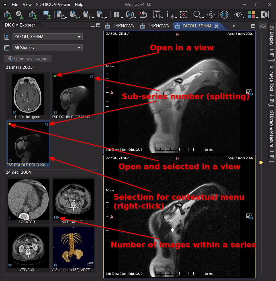
A series is represented by a thumbnail that contains a certain number of images (number displayed at the bottom left).
According to predefined rules, some series are separated into sub-series also represented by a thumbnail with a number preceded by ‘#’ in the upper right corner. Series splitting is necessary for the consistency of some tools such as the MPR, cross-lines and synchronization of series. However, sometimes separation is not desired, and sub-series can be re-merged using the context menu.
The sorting of the series is done by the serial number and if this last one is not present then in a chronological way by the date of the series or other dates.
To open new series:
Drag and drop a thumbnail in the main area (if the series is dropped in a view of the same patient then the series is replaced otherwise a new tab is created).
Double click or navigate with the up/down arrow key and press return on a selected thumbnail (if a view of the same patient exists then the series in the view surrounded by an orange line is replaced)
Select one or more thumbnails and choose an action from the “2D DICOM Viewer” context menu:
Open: Opens the series in the most appropriate layout (replaces the series if the patient’s tab already exists)
Open in new tab: Opens the series in the most appropriate layout in a new tab.
Open in screen: Opens the series in the most appropriate layout in a specific screen.
Add: Adds the series to the current patient’s layout if exists.
Preferences
From the main menu “File > Preferences > DICOM > DICOM Explorer”:
Thumbnail size: defines the width of the thumbnails and adjusts the panel accordingly (Default: 144). It is recommended to restart the application after this change.
Study data sorting: allows sorting the studies by chronological order or inversely chronological (Default: reverse chronology order). Since Version4.1.0.
Open in new tab: behavior to automatically open the images of a patient when using WADO or WADO-RS (Default: All the patients)
Download all series immediately: allows starting the download of the series immediately when using WADO or WADO-RS (Default: true). If unchecked then you must click on the play button on each series or globally at the bottom of the thumbnail list.
DICOM 2D Viewer
Displaying DICOM images
The 2D viewer is the default viewer when opening a DICOM series containing images.
Open the 2D viewer
The 2D view can be opened with
in the toolbar or by right-clicking on the thumbnail in the DICOM explorer.
The rulers K show a real size when it can be calculated from the DICOM file. When a text M above the calibration is displayed, it gives information about the calibration type. Here are some examples:
At dector: The calibration of the projection radiographic image is done at the detector level
Magnified: The calibration of the projection radiographic image is corrected using the magnification factor (e.g. mammography, see the image above)
Used fiducials: The calibration is based on fiducials (e.g. manual calibration with a ruler in the image)
At scanner: The calibration comes from a media which has been digitized (e.g. film digitizer)
Toolbars A
Viewer Main Bar
Select the preferred actions for the three mouse buttons and the mouse wheel:
Mouse left button: The default value is Window/Level. Action can also be changed from the context menu F and the key shortcuts.
Mouse right button: The default value is Context Menu
Mouse wheel: The default value is Series Scroll
Mouse middle button: The default value is Pan
Where the possible actions are:
Pan: Move the image position. T key to select the action. Alt + Arrows keys to pan when another action is selected.
Window/Level: Change the contrast of the image. W key to select the action.
Series Scroll: Scroll through the images of the current series. S key to select the action.
Zoom: Zoom in/out the image. Z key to select the action.
Rotation: Rotate the image with a free angle. R key to select the action.
Measure: Draw a graphic for measuring something. M key to select the action.
Draw: Draw a graphic for annotating. G key to select the action.
Context Menu: Display the context menu. Q key to select the action.
Crosshair: 3D cursor. H key to select the action. Ctrl + click or Ctrl + Shift + click allows changing Window/Level.
No Action: Do nothing. N key to select the action.
Tip
When dragging, accelerate the action by pressing the Ctrl key and Ctrl + Shift to accelerate more.
Default layout: Change the layout of the view. DICOM Information and Histogram are specific layouts where information is automatically updated when scrolling through the series.
Synchronize: The synchronization feature lets you apply the same settings to other images.
None: No synchronization is applied between series.
Default Stack: When selected, the layout is synchronized (window/level, scrolling, zoom) only with the series sharing the same Frame of Reference UID (0020,0052). This is the default behavior.
Default Tile: When selected, the layout is applied in tiled mode (image mosaic of the current series) and is synchronized (window/level, scrolling, zoom) with the image of the same series.
Reset: Reset the image rendering (see below). Escape key to select the action.
Toolbars can be shown or hidden from the View top menu.
Viewer’s tools
Here is a list of the tools which are associated to the DICOM 2D viewer.
The mini-tool is always visible and the other tools are displayed by clicking on the vertical button. The normalize button
allows you to insert the panel into the main layout. Otherwise, the panel is displayed as a popup window with the pin option
(which is not recommended, as it hides other panels).
Mini-tool B
Allows you by default to scroll through the images of the selected series (surrounded by an orange line). From the combobox at the top, the mini-tool can also be configured to change the zoom or the rotation of the image.
Display C
It lets you control the display of the image and the graphic objects.
The Apply to all views option allows you to apply the same display settings to all the views within the selected tab. If unchecked, the display settings are only applied to the selected view (surrounded by an orange line).
Image
Display options for the image. Unchecking the Image option will hide the image and display only the annotations and the graphic objects. The other options are related to DICOM specifications:
Display transformation properties and DICOM information on the image.
Annotations: Display DICOM information on the image corners:
G The top left: Patient information
H The top right: Study information
I The bottom right: Series information (related to the modality type)
J The bottom left: Image information and its position in the series
Minimal Annotations: Reduce the number of annotations. Use space or i key to toggle between the 3 states (minimal, none, all).
Anonymize: Hide identifying information only in the views not in other places of the GUI like the tab title. Must be used with the screenshot tool when exporting image.
Scale: Display the rulers on the left and the bottom of the image K
Allows you to zoom, rotate and flip the image. Zoom and rotation can also be configured with the mini-tool or the mouse actions.
Cine
The Cine start button
lets you scroll through the images in a series at a certain speed (frame per second). The speed values comes from the DICOM file if exists. The cine options can also be changed from the context menu.
Click on Cine stop button
to end the animation.
Click on Loop Sweep toggle button
to change the cine mode: looping vs sweeping.
Note
When the cine is active, the series which are synchronized are also animated. The cine is also applied to other series when they are selected until the Cine stop button is clicked.
When a series have a variable frame rate. The speed is changed automatically. So the speed value entered manually is not preserved.
Tip
A Cine toolbar is also available. It is not visible by default, but can be displayed from the View menu.
Reset
It allows you to return to the default image rendering for all or specific parameters. Also available from the toolbar button
or from the context menu.
From the menu “File > Preferences > Viewer > “2D Viewer”:
Mouse Action Sensitivity
The sensitivity of the mouse drag can be changed according to your preferences for the following actions: Window, Level, Zoom, Rotation and Series Scroll.
Zoom
Zoom interpolation is the process of creating new pixels between existing pixels in an image when it is zoomed in or out.
The Nearest neighbor interpolation is the simplest method. Basically, it extends the pixel value.
The Bilinear method averages the values of the four nearest existing pixels to the new pixel. This produces slightly sharper results than nearest-neighbor interpolation, but it is also slightly slower.
The Bicubic method is similar to bilinear interpolation, but it uses a 16-point kernel instead of a 4-point kernel. This produces even sharper results than bilinear interpolation, but it is also the slowest method.
The Lanczos method uses a sinc kernel to resample the image producing the sharpest results. It is moderately fast, between bilinear and bicubic.
The default value is Bilinear. The Nearest neighbor interpolation is faster but produces aliasing artifacts.
Other
Apply Window/Level on color images: When checked, the window/level is applied on the RGB channels of the image. Otherwise, the window/level has no effect when unchecked.
Inverse level direction: When checked, the level direction with mouse actions is inverted (dragging down will increase the brightness) according to the Basic Image Review profile. Otherwise, dragging down will decrease the brightness when unchecked.
Apply by default the most recent Presentation State: When checked, the most recent Presentation State Object is applied on the related image. Otherwise, it is required to select it from
.
Overlay color: change the color and the opacity of DICOM overlay. The default color is white. The opacity can be changed from the transparency or alpha slider of the different color models in the color picker.
MPR Viewer and 3D cursor
MPR Viewer and 3D cursor (crosshair)
Orthogonal multiplanar reconstruction (MPR)
The orthogonal multiplanar reconstruction (MPR) allows you to create, from the original plane (usually axial), images in the two other planes of the Euclidean space. Only planes along the 3 axes (x,y,z) can be displayed, an oblique plane cannot be obtained with this tool.
The MPR view inherits most of the DICOM 2D viewer properties. It can be opened with
in the toolbar or by right-clicking on the thumbnail in the DICOM explorer.
Note
The menu and the button are only active if the series contains at least 5 images.
When the tab containing the MPR views is selected, the crosshair tool
is automatically applied on the left mouse button. Note that it is possible to change the window/level with the ctrl key while keeping crosshair selected.
By default, zoom and window/level are synchronized between the 3 views. The MRR views can be displayed in different layouts
.
Tip
Once the 2 new plans are created, they also appear in the DICOM explorer and can be exported.
Try to load a volume dataset and open the MPR viewer.
Launch
Info
For more information on the elements related to the orientation of multiplanar views see MPR orientation.
3D cursor (crosshair)
The 3D cursor allows you to synchronize the position of several views sharing the same 3D coordinate system.
In order to know which series sharing the same coordinate system, you can select more than one series from the DICOM explorer by right-clicking on a series and selecting “Select related Series”. Then open the series selection by right-clicking again and selecting “2D Viewer > Open”
The crosshair tool
can be selected in the mouse buttons on the toolbar or by right-clicking on a view.
Try to load several series and select the 3D cursor.
Launch
Preferences
From the main menu “File > Preferences > Viewer > MPR” (Since Version4.1.0):
Auto center axes: Allows you to choose a behavior to recenter the cursor in the different views. The position can be returned to the center systematically with the “Always” option (see the image above) or with the 2nd option only when the position is almost no longer visible (the default value).
Crosshair gap at the center: Defines the size of the empty space in the center of the crosshair
Default layout: The preferred layout used when opening the MPR viewer
Info
The preferences apply to both the MPR and the 3D cursor.
MIP Viewer
Maximum Intensity Projection (MIP)
The MIP viewer is a simple 3D viewer that allows to display the maximum intensity projection of a volume defined by a number of slice of the image stack.
The MIP viewer is also available in the 3D viewer with more advanced options of the volume rendering, but some minimal hardware requirements is necessary.
Open the MIP viewer
The MIP viewer can be opened with
in the Basic 3D toolbar of the DICOM 2D viewer.
Note
If the button is grayed out, it means that the current series has less than 5 images which the minimal number of images for using the MIP viewer.
The MIP Options
This dialog is a modal window that allows you to change the MIP settings and build a new MIP series.
Try to load a volume dataset and open the MIP viewer.
Launch
Note
In MIP mode, the volume is displayed as a 2D projection of the maximum intensity along the perpendicular axis of the image plane. This change in geometry means that overlay graphics are no longer displayed.
Projection type
The projection type defines the way the MIP is calculated. The options are:
Min: Minimum Intensity Projection
Mean: Mean Intensity Projection
Max: Maximum Intensity Projection (the default value)
Slice position
The slice position is used to move around the series to apply the projection and display the result. The Image value represents the position in the series stack.
Slice thickness
The Image Extension value represents the number of slices to use for the MIP calculation. If the images are calibrated and contains the 3D position, the thickness is also displayed in millimeters.
Rebuild Series
It allows you to build a new MIP series according to the MIP options. In this new series the slice position and thickness are modified.
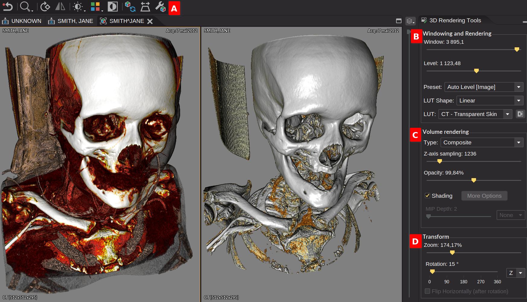
Since Weasis Version4.1.0 the 3D viewer allows displaying volumetric renderings with different options for adjusting the pseudo colors, the transparency, the shadows and the lighting according to the type of exam.
The volume rendering uses a ray casting algorithm and the OpenGL Shading Language (GLSL). Shader programming is used to create the necessary algorithms and data structures
required for the ray casting computations to be executed efficiently on the graphics card. Therefore, minimal graphic resources are required.
Requirements
Some requirements related to the specifications of your graphic card are mandatory. They can be displayed in “OpenGL Support” from the menu “File > Preferences > Viewer > 3D Viewer”:
Driver version: The OpenGL version must be at least 4.3 to support the Compute Shader (not supported currently on macOS)
Max 3D texture dimension length: The limit of any dimension (X,Y,Z) of the volume data
If you have other information in red, it means that the configuration is not optimal but in most cases can work (see how to limit the size of 3D textures)
Note
If the graphic card displayed in Weasis is not the right one, you must solve this problem on the side of the graphic drivers or the operating system.
OpenGL does not include specific functionality for selecting a particular graphics card. Instead, this is handled by the graphics card driver and operating system, which provide a way for users to configure which graphics card should be used by an application.
Open the 3D viewer
The 3D view can be opened with
in the toolbar or by right-clicking on the thumbnail in the DICOM explorer.
Try to load a volume dataset (Medical Demos from data.kitware.com)
Launch
Toolbar A
Actions in the toolbar are:
Allows you to fully reload the volume
The orthographic projection maintains parallel lines unlike the perspective projection that provides a perception of depth. The default mode is the perspective projection.
This tab contains all the tools to modify the volume rendering. If you want to return to the original settings, just click on the toolbar button
or from the context menu.
Windowing and Rendering B
Some of the options described below are also available in the toolbar and in the contextual menus.
Window: The width of a range of voxels values mapped to a specific range of display values.
Level: The center of the range defined by Window.
Preset: Specific values of Window and level. Auto Level [Image] is the default value when changing a LUT and provides the best visual appearance of a Volume LUT.
LUT Shape: The mapping (transfer function) between the input values and the display values can be linear, sigmoid and logarithmic. Default value is linear.
LUT (Volume LUT): A Volume Lookup Table (LUT) is a 3D LUT used to map the grayscale values of a volume dataset to color, opacity and lighting values for visualization. Choosing a LUT from the toolbar or the contextual menu is easier because the LUTs are displayed in an order according to the modality and with a preview.
allows you to invert the LUT.
Volume Rendering C
This panel contains options for the rendering type and its quality, transparency, lighting, and shading settings.
Type: Composite is the classic type of volume rendering. The Maximum Intensity Projection (MIP) is the highest intensity voxels (3D pixels) along a ray path are projected onto a 2D plane. Iso surface is a technique to create a 3D representation on a specific intensity threshold.
Z-axis sampling: The sampling should be large enough to accurately capture the details of the volume data, but small enough to avoid excessive computation time. The default value is calculated according to the size of the volume.
Opacity: The opacity factor of the voxels. Can be set to more than 100% to modify initial values (lower than 100%) transmitted by the Volume LUTs.
Shading: Allows to activate the shading. Default value is defined in LUT. The additional options allow you to override the default lighting settings (comes from Volume LUT).
Transform D
Allows you to zoom and rotate along a specific axis
Preferences
From the menu “File > Preferences > Viewer > 3D Viewer”:
OpenGL Support
Information about the graphics card and OpenGL capabilities, see Requirements.
3D Viewer
Default layout: The preferred layout used when opening the 3D viewer
Max 3D texture size: The maximum size of the volume according to X/Y (width and height of images) and according to Z (number of images in the stack composing the volume)
Note
The maximum values of the default 3D textures come from the graphics card. However, it may be wise to decrease these values (e.g. 512) in order to allow a more efficient display of volumetric renderings for which the hardware resources are not sufficient.
Volume Rendering
Dynamic quality: Allows you to make the render more fluid by reducing its quality (according to the z-axis) when it is rotating or being modified. When the slider is at maximum then there is no more quality reduction.
Default orientation: The preferred orientation used when opening a volume rendering view. Default is Anterior position by turning 15 degrees to the right and 15 degrees downwards.
Background color: Defines the background color of the rendering
Light color: Defines the color of the light during the illumination of the rendering
Video tutorials
Display an MR scan with an angiography-specific protocol by creating a volume rendering. Then either use the MIP type or choose a 3D LUT and adjust the win/level values.
DICOM ECG Viewer
Displaying electrocardiography data
The ECG viewer is used to display and analyze electrocardiogram (ECG) data in DICOM format obtained from different modalities, such as resting ECGs, ambulatory ECGs, and stress tests.
The viewer can also provide tools for measuring ECG intervals and amplitudes in various formats, such as 12-lead ECGs, 3-lead ECGs, and rhythm strips.
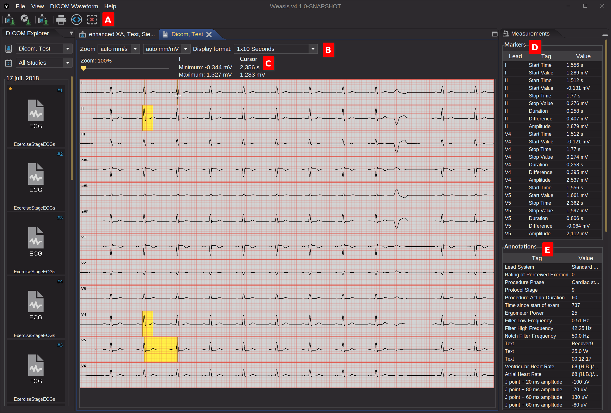
Toolbar A
Actions in the toolbar are:
Allows you to print the ECG as it is displayed with some basic information (patient/study)
Show the DICOM metadata of the ECG
Delete all the measurements (yellow areas in the image above), see Markers
Zoom and Display Format B
The zoom is on several graphic components. The first combo box represents the time, the second represents the voltage, and the slider allows you to zoom in both directions while preserving the aspect ratio.
Time (X-axis): The number of millimeters per second (by default is “auto mm/s”)
Voltage (Y-axis): The number of millimeters per milli-volt (by default is “auto mm/mV”)
The Display Format allows you to show the leads in different layouts.
Lead and Cursor information C
Moving the cursor over the ECG displays the following information:
Lead label: show the minimum and maximum voltage values of a lead
Cursor: show the current time and voltage values under the cursor
Markers D
The markers are the result of the measurements made on the ECG (yellow areas in the image above). A measurement is done by defining a starting and ending point:
Start Time: The time in seconds according to the position of the first point
Start Value: The voltage in milli-volt according to the position of the first point
Stop Time: The time in seconds according to the position of the second point
Stop Value: The voltage in milli-volt according to the position of the second point
Duration: The time elapsed between the 2 points
Difference: The difference in milli-volt between the start value and the end value
Amplitude: The maximum variation in milli-volts from the start value to the end value
The actions for making measurements are:
Action to add a starting point: click
Action to add an ending point: ctrl+click or right-click
Deleting the measurement in a lead can be done by a middle-click or shift+click. Deleting all bars can be done with the button in the toolbar.
Note
Only one measurement is possible by lead.
Annotations E
The annotations come from 2 groups of DICOM metadata:
Acquisition context and Annotations: Attributes which describes the conditions present during data acquisition.
Annotations: may represent a measurement or categorization based on the waveform data, identification of regions of interest or particular features of the waveform, or events during the data collection that may affect diagnostic interpretation (e.g., the time at which the subject coughed).
DICOM SR Viewer
Displaying DICOM Structured Report
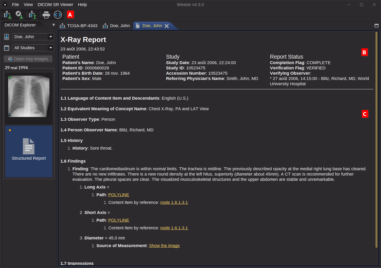
The DICOM Structured Report (SR) viewer is used to display and analyze DICOM SR data. The SR object is a structured collection of content items that represent a report of a diagnostic or therapeutic procedure. The content items are organized in a tree structure, and each item has a relationship with other items.
The viewer displays the content of the SR object in a structured way, allowing the user to navigate through the tree and visualize the content of each item.
The header of the SR object is displayed in a table format with 3 columns containing information about the patient, the study, and the report status.
DICOM SR Tree C
The content of the SR object is displayed in a tree structure. Each node in the tree represents a content item with hierarchical numbering, and the tree structure reflects the relationships between the items.
Some items can have a link to other content items, and the viewer provides a way to navigate through the tree by clicking on the links.
This link can also open a related image which can contain measurements defined in the SR object (e.g. in the image above, clicking on POLYLINE will open the image and display the polyline).
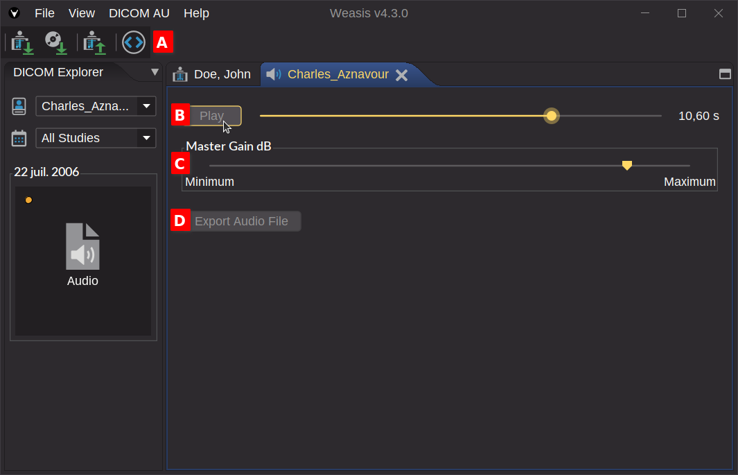
DICOM Audio Player
Playing DICOM AU data
This player is used to play audio data defined by the DICOM AU standard.
For standard images, in an XML File in the same directory of the image (when exporting the images in non dicom file format). The XML file is automatically loaded when the image is displayed in the standard 2D Viewer.
Draw & Measure Panel
When clicking on
of the vertical button
, the panel is displayed on the right side of the viewer. This panel is divided into 4 parts.
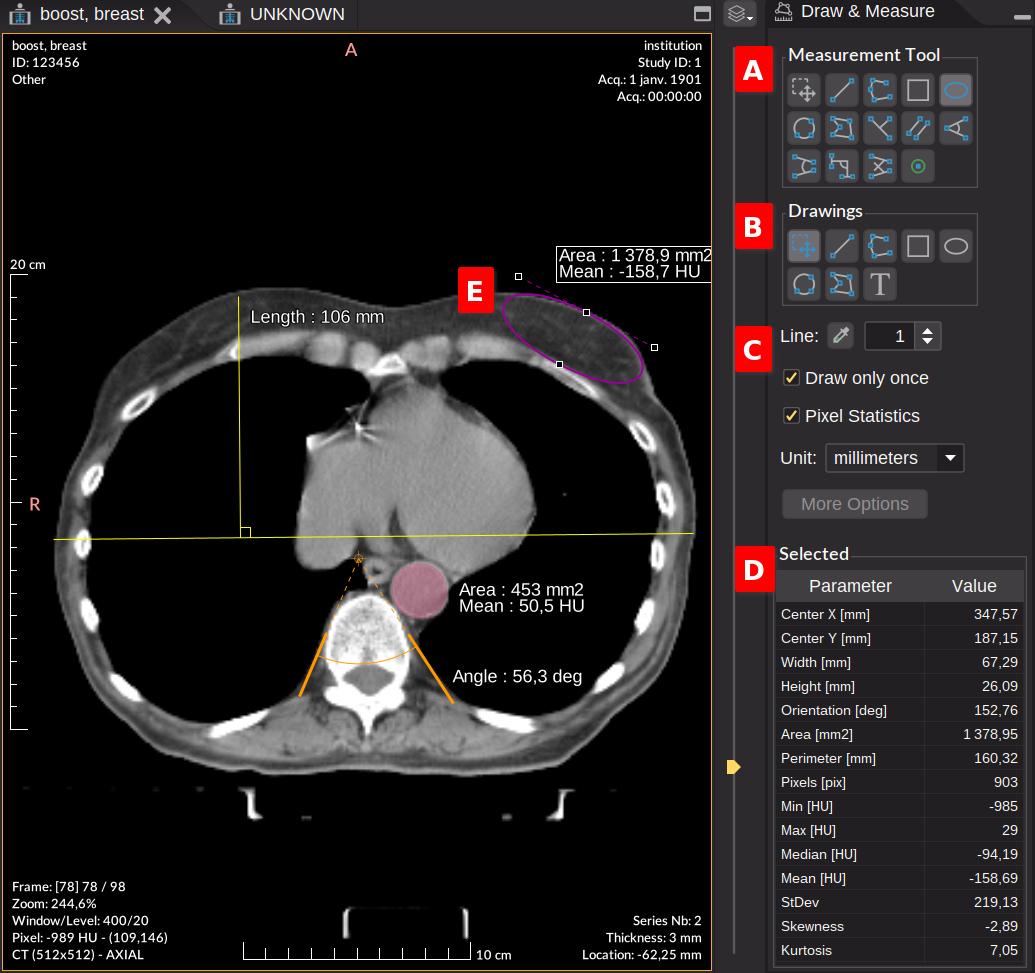
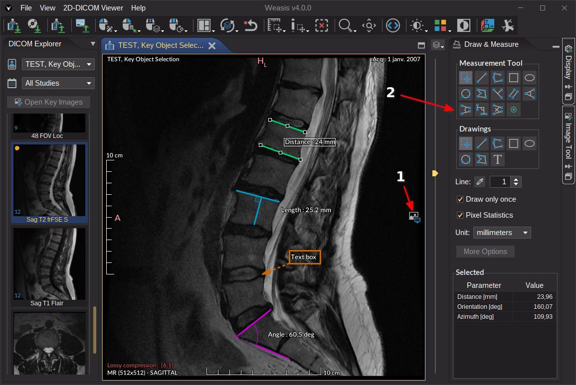
Measurement tools A
Select a measurement tool by clicking on one of the buttons and then draw on the image. Note that the previous action will select automatically the drawing action in the mouse left button.
The first button is the selection tool that allows you to select, resize and move the graphic objects.
By selecting one or several graphic objects, you can change properties (e.g. color, line width) or copy/paste with the contextual menu. You can also delete the selection with the delete key or
. See other shortcuts for graphics.
Note
There are two ways to draw a segment:
Click + drag > release
Click > release > drag > release
In order to continue drawing with the same tool, you can uncheck the Draw only once option (see below).
Tip
For a polyline or polygon, double-click to complete editing. You can also delete a point or add new ones by right-clicking on a specific point.
Rectangles and ellipses can be drawn in any direction. External control points can be used to rotate and resize the shape. With the single control point on the opposite side, you can only resize the shape.
Drawings B
The drawing buttons allow you to add text and graphic as annotations. These graphics objects do not display measurement values and do not appear in Selected MeasurementD.
Graphic Options C
Line color: The default line color when drawing new graphic object. The default value is yellow. The opacity can be changed from the transparency or alpha slider of the different color models in the color picker.
Line width: The default line width.
Draw only once: After drawing a graphic object, the tool is automatically set to the selection mode. If unchecked, the tool remains active for drawing a new graphic.
Pixel statistics: Show statistics of the pixel values within the shape. Only for graphic objects with a closed shape (e.g. rectangle, ellipse, polygon).
More options: The preferences to change more display options (see preferences).
Tip
Show/hide all the graphic objects from the Display panel by checking/unchecking the Drawings option.
Selected Measurement D
The selected graphic E created with a measurement tool is displayed in the table. The table shows the shape properties according to the measurement type (and its units in square brackets if exists).
Note
For polygon, the length, the width and the orientation are calculated with OMBB (Offset Minimum Bounding Box) method which provides a more accurate approximation of the actual length and width based on the bounding box of the polygon.
When Pixel statistics is checked, some statistics are displayed in the table only for graphics with a closed shape (e.g. rectangle, ellipse, polygon). The statistics are calculated from the pixels inside the graphic shape:
Pixels: The number of pixels inside the graphic shape
Min: The minimum modality value
Max: The maximum modality value
Median: The median modality value
Mean: The mean modality value
StDev: The standard deviation is a measure of the dispersion of the values
Skewness: The skewness is a measure of the asymmetry of value distribution
Kurtosis: The kurtosis is a measure of the “tailedness” of value distribution
Note
SUV (Standardized Uptake Value) measurements are added to the table only for PET images containing the required metadata (patient weight,Decay Correction, radio pharmaceutical dose and time…). The SUVs (the minimum, maximum, and average values) are calculated using the body weight (SUVbw) vendor-neutral method.
Tip
The table can be exported by copy/paste. Note that the maximum precision values are copied and not the rounded values displayed in the table.
Preferences
From the menu “File > Preferences > Draw & Measure”:
Drawings
It lets you change the graphic properties when drawing new graphics, since Version4.3.0.
Line color: The default line color. The default value is yellow. The opacity can be changed from the transparency or alpha slider of the different color models in the color picker.
Line width: The default line width.
Fill shape: When checked, the shape is filled with the line color.
Fill opacity: The opacity of the interior of the shape, relative to the opacity of the line color. The default value is 100%. For example, if the line color has an opacity of 80% and the fill opacity is 20%, then the perceived opacity will be 16% (0.8 * 0.2).
Labels on image
It lets you change the display options for labels attached to measurement graphics.
Font type: The default font size of the labels on the image. The default value is Small semibold. Note that the font size is not absolute and is automatically adjusted according to the scale factor.
Geometric measurement: the measurement types displayed on the image according the graphic type.
Pixel statistics: the statistics types displayed on the image for graphic objects with a closed shape (e.g. rectangle, ellipse, polygon).
DICOM RT Tools
Displaying radiotherapy information
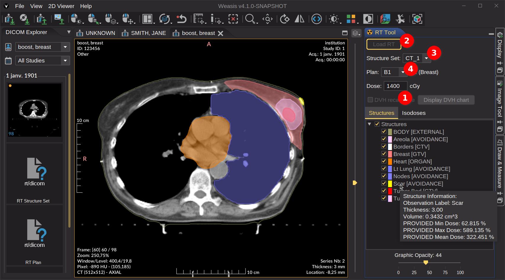
The RT Tool appears on the right panel when a CT exam (when linked with DICOM STRUCT, PLAN and DOSE) is displayed. Since Version4.1.0 a specific configuration in config.properties is no longer required.
How to display structure and iso-dose
In order to display the structures in overlay on the image, apply the following points (see in the image below):
InfoOptional When selected, it allows you to force the DVH calculations. Otherwise, it is calculated only if some information is not available in the DICOM files.
Click on “Load RT” button to load DICOM STRUCT, PLAN and DOSE associated the CT images. Once loaded, the button becomes inactive.
InfoOptional Select a structure if there is more than one.
InfoOptional Select a plan if there is more than one.
Note
The “Structures” tree has the same options as DICOM SEG regions, see DICOM Segmentation.
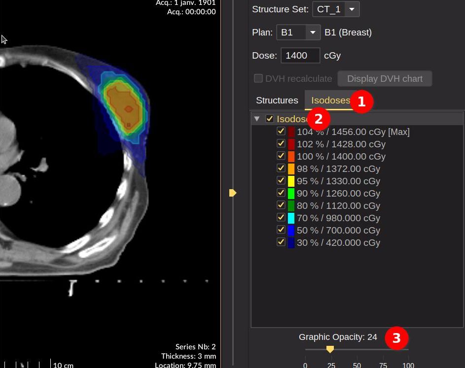
For displaying the iso-doses, apply the following points (see in the image below):
Select the Isodoses tab
Check the Isodoses root node which is not activated by default
InfoOptional Adjust the graphic opacity
Tip
The “Structures” and “Isodoses” root node can be used to show or hide all graphics while the child nodes can be used independently for showing specific items.
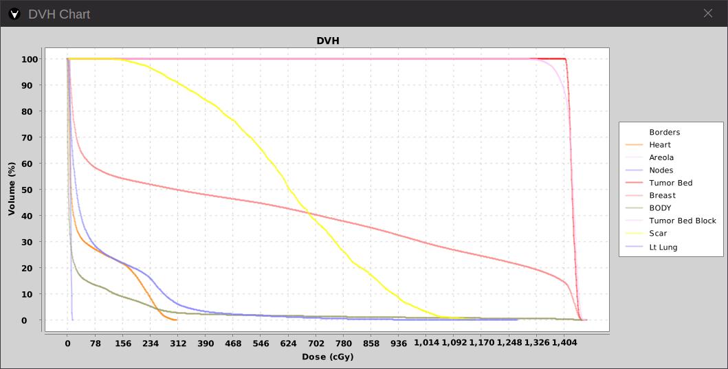
How to display DVH
Select one or several structures. Note: the Structures root node must be selected.
Click on the button “Display DVH chart”
Right-click on the chart to print or save as a PNG image or vector files such as SVG or EPS.
DICOM Attributes
How to display DICOM attributes
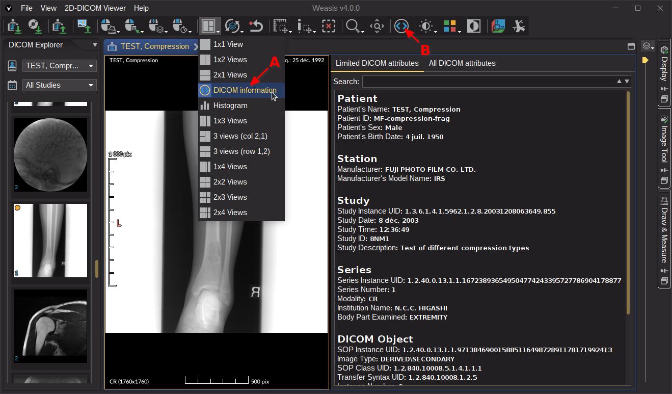
The DICOM attributes
can be displayed either by:
selecting the “Dicom Information” layout from the layout dropdown button A
clicking on the “Dicom Information” button in the toolbar to open a detached window B
Note
Using the view in the layout (A) allows updating dynamically the DICOM attributes to the current image (e.g. scrolling into the series). The DICOM attributes won’t change when opening the detached window (B).
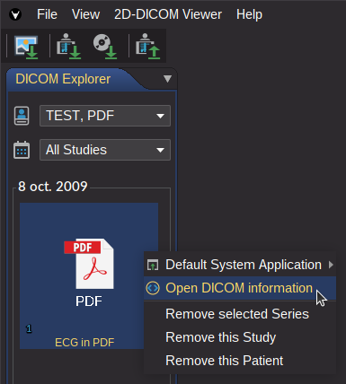
When Weasis opens particular DICOM files (e.g. PDF and video) with an external viewer, the DICOM attributes can be viewed from the thumbnail context menu (see image below).
How to find a specific DICOM attribute or value
The Dicom Information window contains two tabs:
Limited DICOM attributes: List of the main attributes assembled in several groups.
All DICOM attributes: List of all the attributes where each data element is displayed within four columns (Tag ID, VR, Tag Name and Value)
Note
When the data element contains several values, each value is separated by ‘\’.
Data element with a value representation (VR) OB, OD, OL, OF, OW and UN shows “binary data” as value.
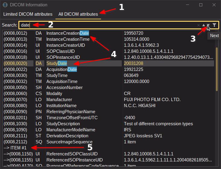
In the image above, we are looking for the word “date”. Here are the steps:
Select All DICOM attributes tab for having all the attributes.
Enter the word you are looking for.
Use the arrows to navigate into the highlighted results. The button on the far right allows you to limit the results to positive ones.
The navigation shows the current result in highlight mode.
Using in the toolbar allows you to filter the results. This can be useful to keep the focus on certain elements when scrolling through a stack of images (only possible with layout A).
Note
Some attributes can be into a sequence element (5). Note: the left arrow shows the depth level as a sequence can contain another sequence.
Tip
If there isn’t enough space to display the entire value, simply resize the column from the header (only persistent if the image doesn’t change) or use tooltips by positioning the cursor over the elements (since v4.3.0).
Tip
The DICOM attributes can be copied into the clipboard with the copy shortcut of your system.
Lookup Tables (LUT)
How to handle Color and DICOM LUTs
A DICOM file can contain one or more LUTs. The DICOM pipeline for rendering images contains a number of stages where the LUTs are applied. There are 4 types of Lookup Tables (LUTs) in DICOM:
The Modality LUT is used to transform the pixel values into the values of the modality (e.g. Hounsfield for CT).
The Values of Interest (VOI) LUT is used to transform the modality values into a visible range that enhances specific anatomical structures or pathological conditions.
The Presentation LUT is used to transform the intensity values into P-Values (presentation values are device-independent values related to human perception).
The Palette Color LUT is used to transform the intensity gray values into color values with a pseudo color LUT.
Note
The Modality LUT and the Palette Color LUT are applied automatically when they exist. There are no options in the User Interface to modify them.
Windowing and Rendering
The Windowing and Rendering is a panel in the Image Tools of the DICOM 2D viewer. Some of the options described below are also available in the Lookup Table toolbar, in the main menu and in contextual menus.
Window: The range of pixel intensity values. The value can be changed when Window/Level is selected in mouse actions or by using the slider.
Level: The center of the range defined by Window. The value can be changed when Window/Level is selected in mouse actions or by using the slider.
Preset: The possible items ordered according to the following list:
Empty item when the Window and level values are changed manually from slider or mouse actions.
Window and level values or VOI LUT data from the DICOM file (ending with [DICOM]). The default value is the first [DICOM] item if exists, otherwise Auto Level [Image].
Auto Level [Image] (always visible) which is the Window and level related to the full range of the pixel values
Specific values of Window and level for a modality type (e.g. Lung for CT)
LUT Shape: The mapping (transfer function) between the input values and the display values can be linear, sigmoid and logarithmic. Default value is linear.
LUT: A pseudo color LUT used to map the grayscale values to color. Default (image) is the original image color model. Choosing a LUT from the toolbar or the menus is easier because the LUTs are displayed with a preview.
allows you to invert the LUT.
Filter: The 2D filter is applied to the image before the LUT. The filter can be used to enhance the image quality or to highlight specific structures. The default value is None.
Tip
In order to display the LUT on the image, select it from the Display panel on the right. The LUT color are associated to values that correspond to the Modality LUT values (e.g. Hounsfield values for CT) or to the pixel values for some imaging types.
Another way to see the windowing transformation is to display the histogram.
Build DICOM KO and PR
How to build and export DICOM KO and PR
Key Object Selection (KO)
In order to display KO Toolbar, select in the main menu: View > Toolbars > Key Object Selection Toolbar
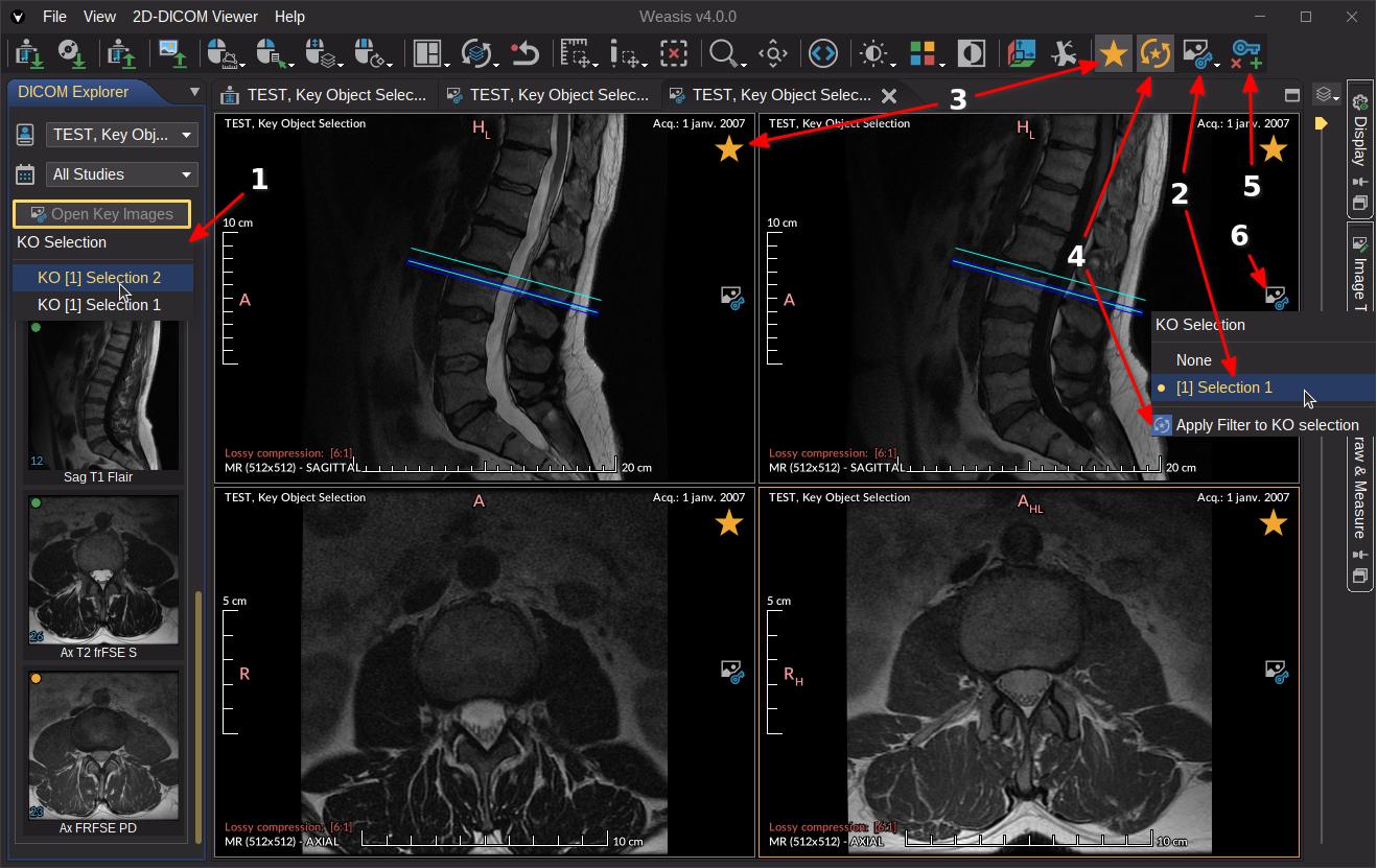
When a DICOM KO is loaded then it appears in the explorer menu (1) or it can be selected from the icon on the right of the view (6).
Click on the star icon (3) to add the key image or press ‘k’ to create in a new KO.
Other actions:
Apply a KO (2)
Filter to obtain only the key images defined in the selected KO (4). This means only key images will be visible when scrolling into a series.
Create a new KO (or based on another one) or delete KO (only the ones created by Weasis) (5)
Presentation State (PR or GSPS)
Apply PR loaded from a DICOM file (1)
: Since Version2.6.0 PRs are not applied to the image by default (requires to select the right icon (2) over the image). In order to apply the most recent PR by default, change it from the main menu File > Preferences (Alt + P) and check “Apply by default the most recent Presentation State”, or in the default preferences.
Create a new PR: Any type of annotations (Drawings and Measurements) can be exported in a DICOM Presentation State. Image presentation actions (zoom, calibration, W/L, LUT…) are not yet possible to export into PR.
Exporting Key Object Selection or Presentation State
In order to export KO or PR, select the DICOM Export icon or from the main menu File > Export > DICOM
Select the export type (locally or remotely)
Choose the exporting options (series created by Weasis have the flag “NEW”)
Select the patient/study/series/instance to export
Export the selection and close the Window
DICOM SEG
Displaying DICOM Segmentation
Since Weasis Version4.3.0, this panel lets you display the contents of a DICOM SEG file superimposed on the image. It also lets you modify the transparency of specific regions (label defined by a color).
DICOM SEG can be generated by AI frameworks to represent the results of segmentation algorithms applied to medical images.
How to display DICOM SEG
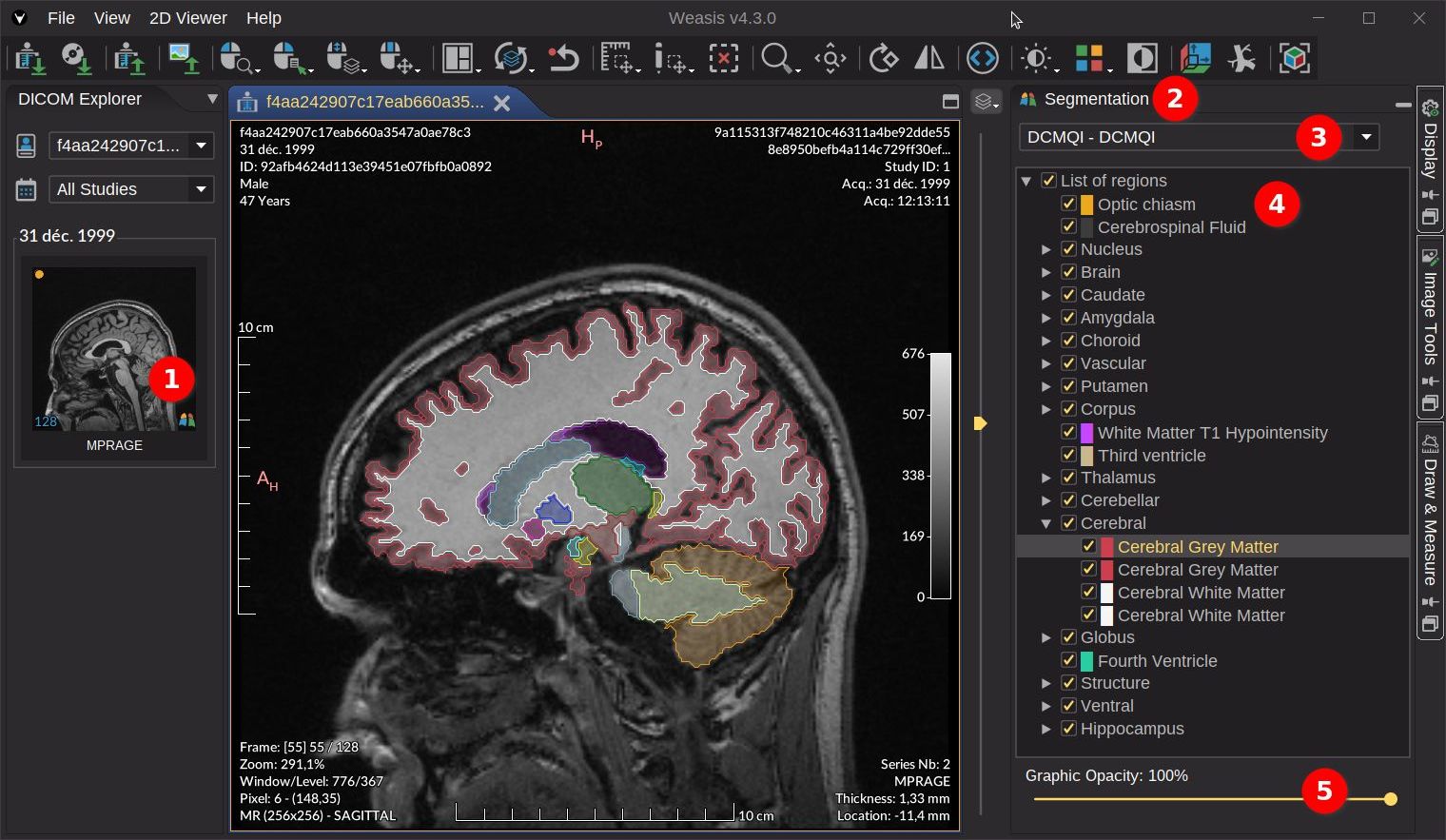
In order to display the DICOM SEG regions in overlay on the image, follow these steps (see in the image below):
Open the DICOM series with a link to a DICOM SEG object. This link is visible by the segmentation icon
in the lower right-hand corner of the thumbnail.
Once the image is displayed, you can click on
of the vertical button
to show the Segmentation panel on the right side of the viewer.
A DICOM SEG file is represented by a selected item in the combo box and its list of regions below. By default, all DICOM SEG files linked to an image are displayed.
Select one or several regions to display for the selected DICOM SEG (3). Several regions are grouped together when they share the same first name. Note: the parent node must be selected to display the child regions.
Adjust global graphic opacity (border and interior)
Note
The regions tree has context menus that allow you to:
Fill opacity (all nodes): The opacity of the interior of the shape, relative to the opacity of the line color (Graphic Opacity). The default value is 20%. For example, if the line color has an opacity of 80% and the fill opacity is 20%, then the perceived opacity will be 16% (0.8 * 0.2).
Select/Unselect all the child nodes (only for parent nodes)
Show ih the images view (only for leaf nodes): The region with the highest surface area is displayed in the image overview.
Pixel statistics from the selected view (only for leaf nodes): Show statistics of the pixel values within the region shape. For the definition of the statistics parameters, see graphic Pixel Statistics.
Tip
The regions tree has tooltips on leaf elements that show the region description and the region volume.
AI DICOM Objects
DICOM objects generated by artificial intelligence
Artificial intelligence (AI) frameworks can produce various DICOM objects for different purposes. Here are some common DICOM object types produced by AI frameworks and how they are handled in Weasis (see Info window).
DICOM Secondary Capture (SC)
This type of object represents secondary images where the AI has embedded information in the image pixels. These images may include annotations, measurements, or other enhancements to the original image data.
Info
DICOM Secondary Capture can be displayed by Weasis like any other image data, see DICOM 2D Viewer.
DICOM Segmentation (SEG)
These objects represent the results of segmentation algorithms applied to medical images. Segmentation involves partitioning an image into multiple segments to simplify its representation for analysis or display. AI frameworks can produce SEG objects containing segmentations of anatomical structures, lesions, or other regions of interest.
Info
See DICOM SEG for displaying DICOM SEG objects in Weasis.
DICOM RTSTRUCT
This type of DICOM object is originally used to represent structures delineated on CT images for radiotherapy treatment planning. Some AI frameworks may produce DICOM RTSTRUCT objects (geometric shapes) instead of DICOM Segmentation (pixel-based).
Info
See DICOM RT for displaying DICOM RTSTRUCT objects in Weasis.
TotalSegmentator automatically segments over a hundred anatomical zones on CT images.
When the result is saved in DICOM RTSTRUCT (since version 2), the segmentation result can be displayed directly in Weasis:
DICOM Structured Report (SR)
AI frameworks can generate structured report containing the results of their analysis. These reports typically include structured information about findings, measurements, observations, and interpretations derived from medical images or other data.
AI frameworks may produce DICOM objects containing encapsulated documents such as PDF reports, text documents, or other non-image data related to medical imaging studies.
Info
This type of object can be displayed by the default system application associated with the document mime type. The DICOM attributes can be viewed from the thumbnail context menu (see image below).
DICOM Presentation States
Presentation states define how images should be displayed, including display parameters such as window width, window center, and image orientation. A Grayscale Softcopy Presentation State (GSPS) object is used to display annotations and graphics that overlay on a displayed image. AI frameworks might generate presentation states to specify how images should be displayed based on their analysis results or to display graphics overlays on images.
Info
See DICOM PR for displaying DICOM Presentation States in Weasis.
DICOM Enhanced Objects
Enhanced DICOM objects contain additional information. AI frameworks might produce enhanced DICOM objects to include additional annotations or other enhancements to the image data.
Info
DICOM Enhanced (e.g. reduce noise or improve visualization of anatomical structures) can be displayed by Weasis like any other image data. Some other additional information (overlay, shutter and pixel padding) can be added to the image rendering, see 2D Viewer Display.
Zoom
Zoom tool
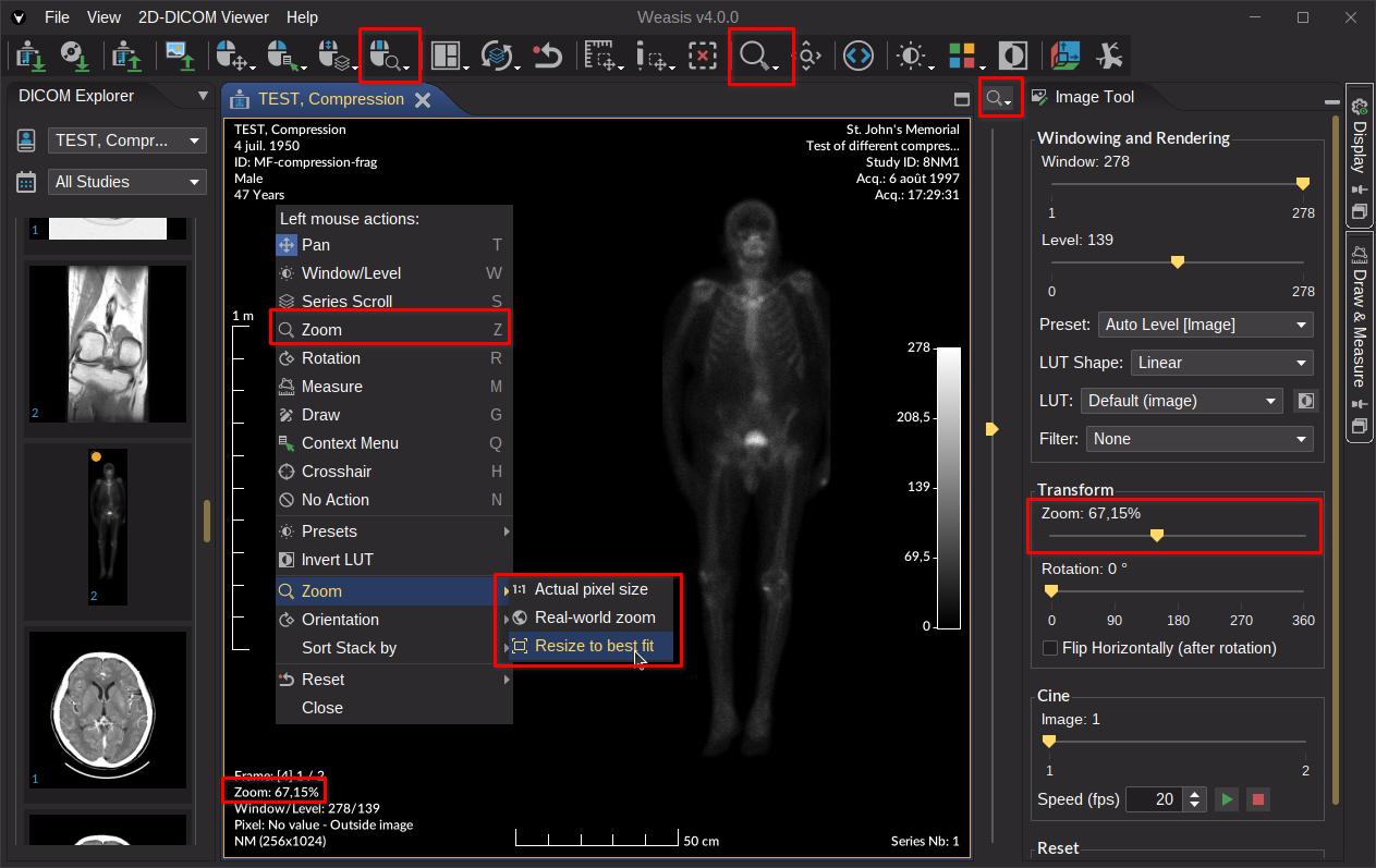
The zoom tool can be associated with one of three mouse actions . In the image below the zoom tool
is associated with the middle mouse button. See also zoom preferences.
The zoom factor can be modified from different locations:
By dragging the cursor over the image with the configured mouse button
By scrolling the mouse wheel when configured
By selecting an item in the zoom dropdown button in the toolbar
From the context menu: right-click on the image > Zoom
Form the slider in the image tool panel
Using Keyboard Shortcuts (Ctrl + Plus (+), Ctrl + Minus (-) and Ctrl + Enter) on the selected view
The context menu and the toolbar button allows you to select different zoom factor:
Actual pixel size
: display the image at a 1:1 ratio, where each pixel in the image corresponds to one pixel on the screen
Resize to best fit
: scaling the image to make it fit the view area as closely as possible
Note
The zoom function always zooms in/out to the center of the screen regardless of where the cursor is. This mode provides greater positional accuracy in particular situations.
Since “Resize to best fit” is the default mode for a view, the image will be centered when scrolling to the next image. You need to change the mode or the zoom factor to keep the image off center when scrolling.
Tip
For selecting directly the zoom action of the mouse left button, enter “z” as a shortcut.
Real-world zoom
The real-world zoom allows displaying the content of the image at the same size of the real objects.
The feature requires calibrating the screen where the image is displayed. From the main menu, open File > Preferences (Alt + P) > Monitors and click on Spatial calibration. Then enter a value that matches to the line length or the diagonal length of the screen.
Note
Several screens can be calibrated. Each one has its own spatial calibration factor.
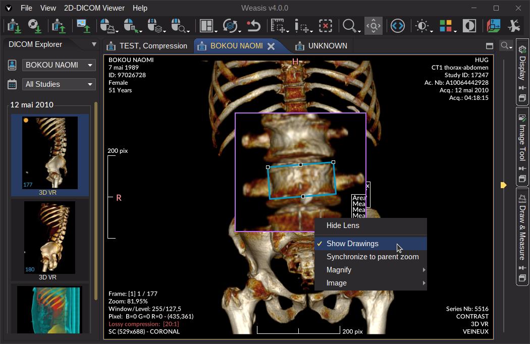
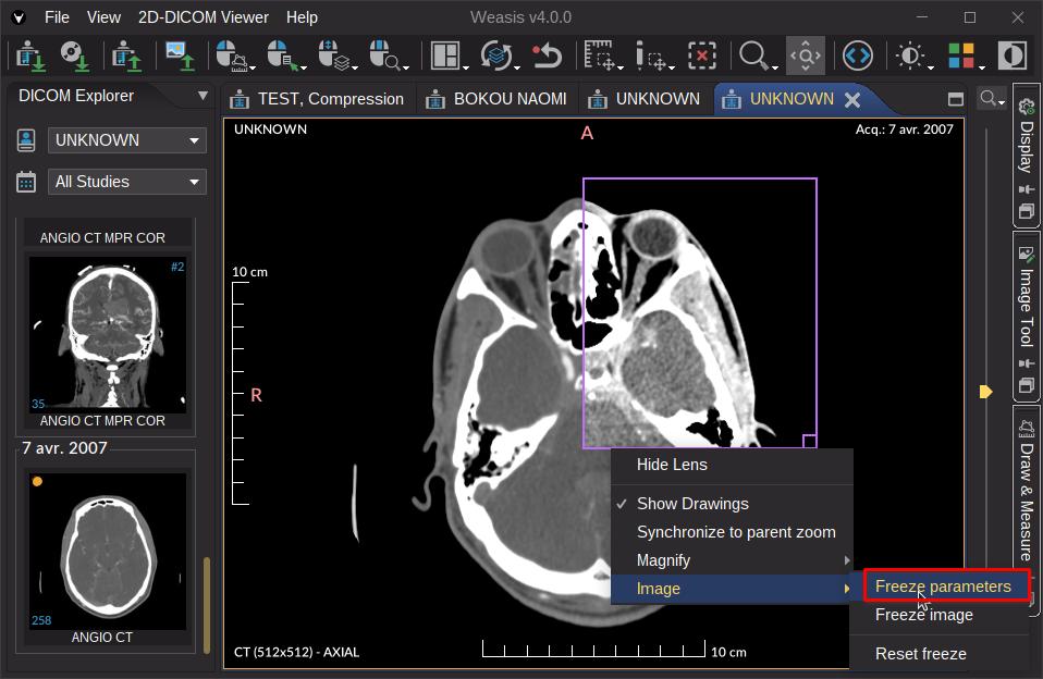
Magnifying lens
The magnifying lens can be activated from the toggle button of the zoom toolbar (see the image below). It has several parameters accessible from the context menu.
This lens can be used in many situations, for instance:
to magnify a specific area
to compare two images from the same series (select Freeze image)
to display a specific area without the drawings (Unselect Show Drawings)
to compare different values of Window/Level (select Freeze parameters - see image below)
Note
Using the mouse wheel on the lens changes the zoom factor. Double-clicking on the lens adjusts the zoom factor of the lens to the one of the main image.
Parameters of the context menu:
Synchronize to parent zoom: When this option is activated, the zoom factor of the lens is permanently adjusted to the zoom factor of the main image (meaningful when using freeze parameters).
Show Drawings: Displays in the lens the visible drawings.
Magnify: Allows to select a zoom magnitude.
Image:Freeze parameters allows you to keep the current image processing (c.f. Window/level, LUT or filter) and Freeze image allows you to keep the current image and its parameters.
Histogram
Displaying Histogram
Displaying the histogram allows you to view the distribution of the modality values.
Note
Displaying the histogram allow you to better understand the effect on the pixel distribution wen changing all the LUT parameters from the Image Tool right panel.
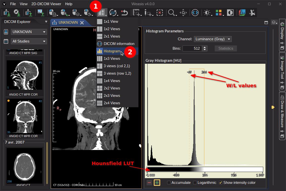
To open the histogram, select the “Histogram” layout from the Layouts dropdown button (see the image below).
General histogram parameters:
Channel: With gray images only the Luminance channel is available. With color images, you can choose one of the following color models: RGB, HSV and HLS.
Bins: The bins are the intervals values of pixels. By default, this number is calculated by the max value minus the min value and cannot exceed 512. The value entered must be between 64 and 4096.
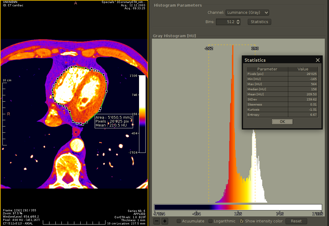
Statistics: Show the statistics of the histogram which allow you to analyze and to compare images or image regions in a quantitative way. For the definition of the statistics parameters, see graphic Pixel Statistics.
Note
The values on the x-axis represent the modality values (e.g. Hounsfield for CT) or the pixel values for some imaging types. If the unit of the pixel value of the modality exists, it is visible at the end of the histogram title.
Display histogram parameters:
-/+: shrink/strech the y-axis scale (the number of occurrences)
Accumulate: Display a cumulative histogram
Logarithmic: Show the number of occurrences in a logarithmic scale (y-axis).
Show intensity color: Show the bin with the LUT colors, otherwise in black.
Reset: Set the default parameters
Note
It is possible to display the histogram of a region with the measurement tools. Simply select the region to display its histogram (see the image below).
Tip
Clicking on the histogram bin allows displaying the number of occurrences and the modality range values of the selected bin.
Image orientation
Interpretation of the orientation
The orientation of the DICOM images is displayed by one or more uppercase letters in the middle on the top and left of the view.
If Anatomical Orientation Type (0010,2210)attribute is absent or has a value of BIPED, anatomical direction is:
A: anterior
P: posterior
R: right
L: left
H: head
F: foot
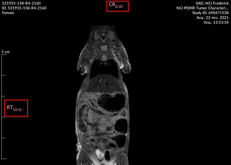
If Anatomical Orientation Type (0010,2210)attribute has a value of QUADRUPED (since Version4.1.0), anatomical direction is designated by:
LE: Left
RT: Right
D: Dorsal
V: Ventral
CR: Cranial
CD: Caudal
R: Rostral
M: Medial
L: Lateral
PR: Proximal
DI: Distal
PA: Palmar
PL: Plantar
Info
If the orientation is not perfectly aligned according to the 3 axes of the referential then there can be a secondary and tertiary orientation (in subscript) separated by “-”.
Info
For some modalities such as CR or DX, the orientation comes from the Patient Orientation (0020,0020) attribute and is not displayed when using the rotation tools because it cannot be recalculated dynamically.
For other modalities such as CT and MRI, the orientation is always displayed because it is dynamically calculated.
Tip
To display or hide the orientation on the image, select it from the Display panel on the right (DICOM Annotations > Orientation).
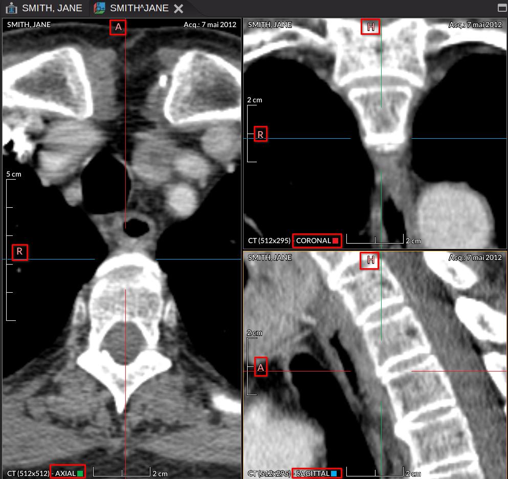
Orientation in 2D multiplanar reconstruction (MPR)
The image below shows the 3 views of the orthogonal MPR. The uppercase letter at the left or at the top designates the orientation of each multiplanar view whose type (axial, coronal, sagittal) is defined at the bottom.
Info
The color of the axes used comes from the one defined in DICOM Patient Orientation. Blue corresponds to the left-right axis, the red axis to anterior-posterior, and the green axis to foot-head.
The colored square in the MPR view above corresponds to the plane that is perpendicular to one of the axes.
Print
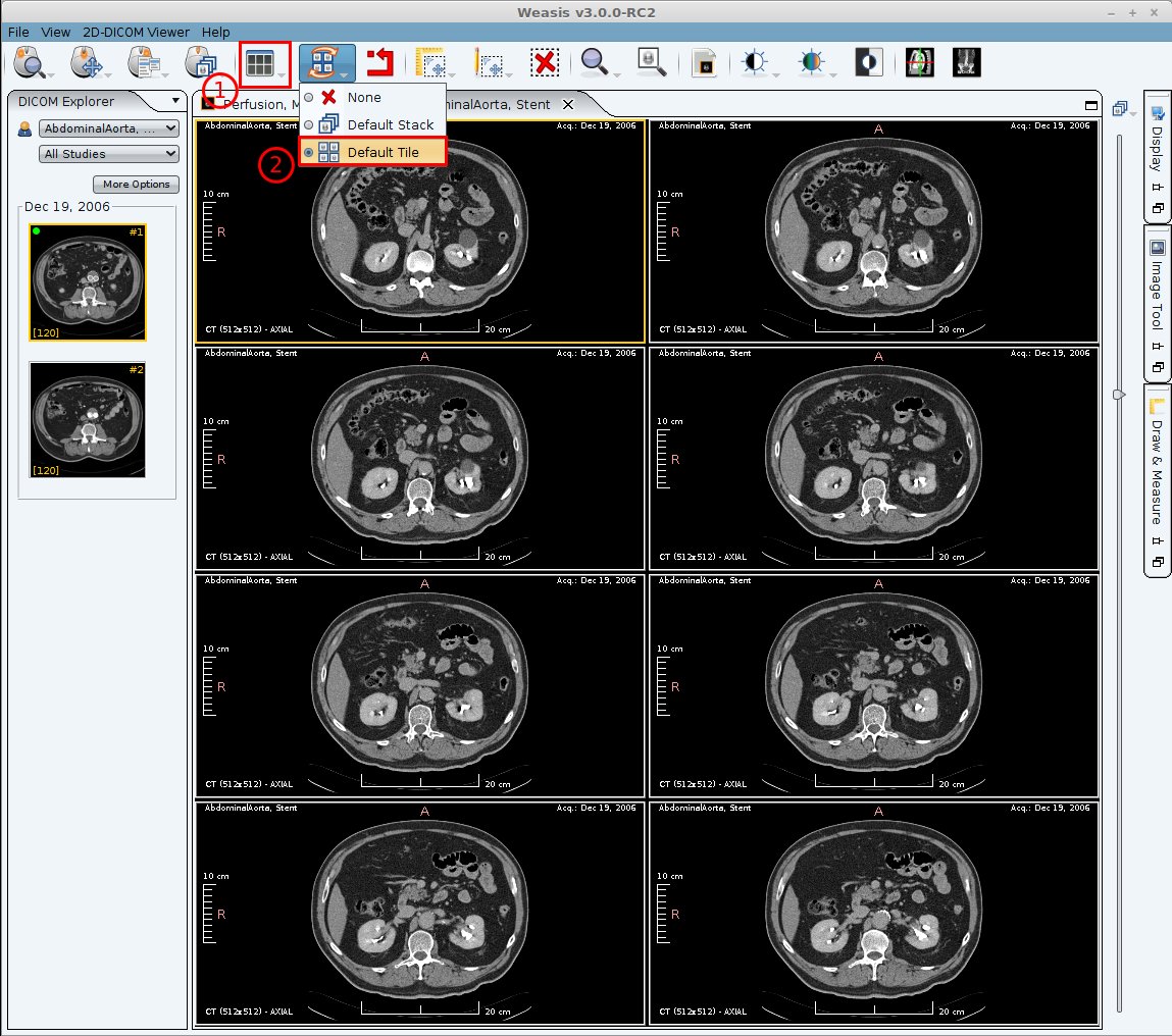
Build the image selection to print
The image selection to print must be prepared before calling the print function. If you need to print more than one image per page, choose a layout from the dropdown button in the toolbar (1).
Note
The layout list is built dynamically according to the window size. So changing the window size ratio will provide other layouts. For instance, with a panoramic screen, you can choose a horizontal layout and then print with a landscape orientation.
To fill the layout with images you can change the synchronized mode of series (2):
with Default Tile selected, all the views will be filled with the same series. Each view has a new image of the series stack (n + 1).
with Default Stack selected, drag and drop a series into each view and select independently which image you want to display.
Select a print mode
Standard Printer
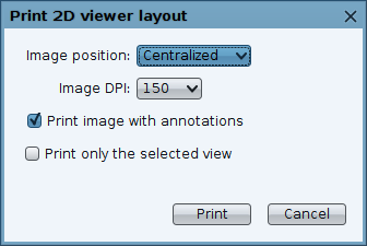
From the main menu, open File > Print > Print 2D viewer layout (P).
The meaning of the standard print parameters:
Image position: the position of the image in the print area.
Image DPI: the print resolution in dot per inch (Default value is 150). Higher DPI means higher resolution.
Print image with annotations: Allows to print the annotations defined in the Display panel.
Print only the selected view: When this option is checked, only the selected view is printed (view with an orange border). Otherwise, all the views of the layout are printed.
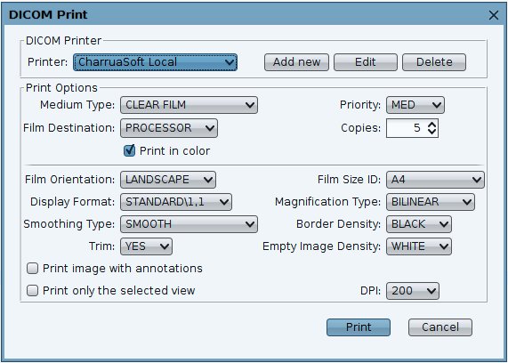
DICOM Print
From the main menu, open File > Print > DICOM Print.
In the DICOM Print dialog, you can manage several configurations. For the options meaning, you can refer to the above parameters and the DICOM print pages.
Note
The DICOM printer configurations can be distributed at the server side for all the clients, see preferences.
Spatial Calibration
How to change the spatial calibration
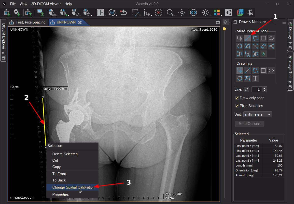
When the image does not contain a default spatial calibration and it contains a ruler (or other element allowing to determine a known distance) then you can apply a calibration manually:
Select a line in the Measurement Tool
Draw a line on an object with a known distance
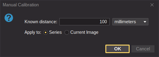
Right-click on the selected line and enter the distance on the Manual Calibration window
Note
The calibration can be applied only to the current image or to all the images belonging to the series.
Info
Once calibrated, all measuring tools will produce results according to the calibration and the real-world zoom will display the images at the same size of the real objects. Currently, the calibration is not saved in the DICOM file.
Changing spacial calibration with Weasis 1.1.3
Styles and themes
Change the appearance of the user interface
How to apply another theme
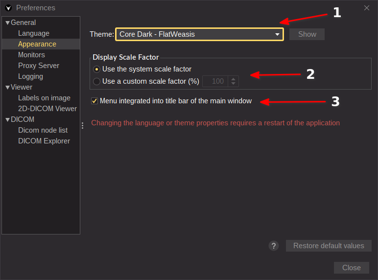
From the main menu, open File > Preferences (Alt + P) and select the desired theme and click on “show” to see a partial preview (1).
How to scale the user interface
It is recommended to adapt the scale factor to the one of the system (2). In this way, Weasis will scale on HiDPI displays as the operating system. On Windows it is the Display Scaling preference and on Linux it is either the display scaling factor or the text scaling factor.
However, the scaling factor can be increased (or even decreased) independently of the system. That means all the elements of the graphical interface will be adapted (fonts, icons, graphic components…).
Note
The last option (3) allows you to force the integration of the main menu in the window bar (not activated by default). This option appears only on Linux because there is a wide variety of window managers.
On Windows and Mac this option does not appear because it is always supported.
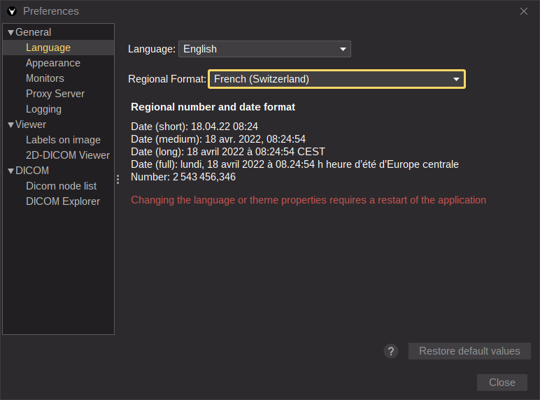
From the main menu, open File > Preferences (Alt + P) and select the desired language and the regional format. The languages available in the list can be partially translated. In this case you can participate in the translation directly from a web portal.
Note
Anywhere in the user interface, date and number should be displayed with the selected regional format.
Changing the default locale settings
If you need to change the default settings, please see the preferences.
Logging
Configure and view log files
The log folder that can be opened from the menu “Help > Open the logging folder” (since Version4.1.0) contains two types of log:
A boot log file (boot.log) is always written since Version3.5.0
Rolling log files (default.log) that need to be activated in the preferences dialog (see below How to configure the rolling log files)
Tip
In order to determine the path of <user.home>/.weasis/log for versions prior to v4.1.0, go to the “Help > About Weasis” menu and find the property weasis.path in the “System Information” tab.
Boot log files
The boot log file is used to trace the startup configuration to ensure that the application starts with the correct input parameters and configuration.
This type of logs is interesting if the application doesn’t start, crash at startup, or if there is a problem with the startup preferences.
How to configure the rolling log files
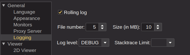
From the main menu “File > Preferences > General” enable “Rolling log” to activate writing to files
Enter the maximum of File numbers for rolling log (by default 5)
Enter the maximum size of each rolling file (by default 10 MB)
Select a log level which defines the verbosity of the traces (by default DEBUG)
Select a stacktrace limit which represents the number of lines (by default no value). No value is recommended for investigating problems (it means unlimited stacktrace lines)
Info
The default logging configuration comes from config.properties or ext-config.properties, see Weasis Preferences.
Proxy server
How to configure a proxy server
Manual configuration from the user interface
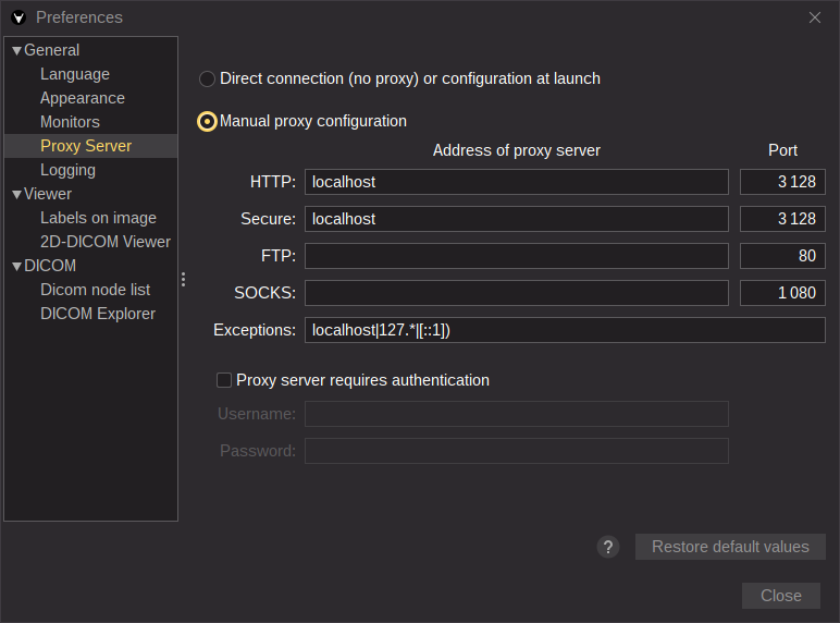
From the main menu, open File > Preferences (Alt + P) and select Proxy Server.
The default configuration is Direct connection (no proxy) and by clicking on Manual proxy configuration you can define a custom proxy server (in the image below, a local proxy like Squid).
In order to fill in the fields, you must refer to the Java documentation.
Tip
In some cases it is necessary to restart Weasis.
Configuration at launch
For setting JVM properties at launch, the selection in user interface must be Direct connection (no proxy) or configuration at launch.
Tip
The Java options can be manually set in the section “[JavaOptions]” of Weasis.cfg (in the installed path).
The Java options can also be passed in the parameters of the URL (e.g. http://localhost:8080/weasis-pacs-connector/weasis?patientID=9702672&pro=“https.proxyHost%20127.0.0.1”&pro=“https.proxyPort%203128”).