Weasis provides the tools to visualize and analyze images obtained from medical imaging equipment according to the DICOM standard. This free DICOM viewer is used by healthcare professionals, researchers and patients.
If you are new to Weasis, it is recommended to read this page to understand the main elements of the interface.
The tutorials are organized by topics and can be read independently.
If you find any errors or inaccuracies, just click the Edit button displayed on top right of each page, and make a pull request to submit your changes.
Subsections of Tutorials
GUI Overview
Essential aspects of the interface
The image below shows the main elements of the Weasis graphical user interface. Click any of the green or blue areas to jump to the dedicated documentation for that element.
The default DICOM workspace has two main areas:
The DICOM Explorer on the left (blue) — used to import and export data and to pick the series to display.
The main area on the right (green) — hosts the open viewers and players as tabs. The available menus, toolbars, and tools change depending on the viewer currently in focus.
In the screenshot above, the active viewer is the DICOM 2D Viewer
, which is the default for image series.
A tab with a multi-view layout can only display images from a single patient, but the same patient can appear in several tabs.
Each tab is a docked panel that can be moved by drag-and-drop, including side-by-side splits — see Docking for the full layout options.
For navigating through the Patient / Study / Series / Image hierarchy, see the DICOM Explorer page.
Minimal configuration before starting
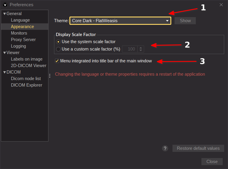
A few settings make Weasis noticeably more comfortable the first time you launch it. Open the preferences dialog from the main menu: File > Preferences (Alt + P).
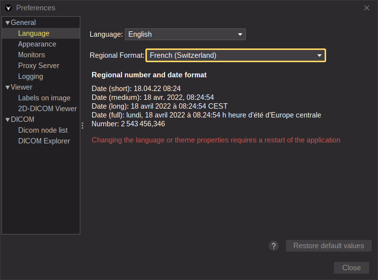
Language and regional settings
In the General tab, pick your preferred language and regional format (dates, numbers). Only languages with at least 30 % translation coverage appear in the list. Dates, numbers, and other locale-sensitive values follow the selected regional format throughout the interface.
Choose a theme that suits your environment and reduces eye strain. The recommended theme is Core Dark — Flat Weasis.
Set a scaling factor that matches your system display scaling. This is especially recommended for HiDPI screens — Weasis will scale fonts, icons, and every UI component consistently.
Wherever you need more complete instructions, click the button in the preferences dialog or in any contextual pop-up — it opens the matching page of this documentation in your browser.
Tip
In the View menu at the top, the toolbars and tools attached to the active viewer can be shown or hidden. These preferences are remembered across restarts. Show / hide preferences specific to the DICOM Explorer are only kept for the current session.
Other viewers and players in the DICOM workspace
Depending on the SOP Class of the loaded series, Weasis opens one of the following:
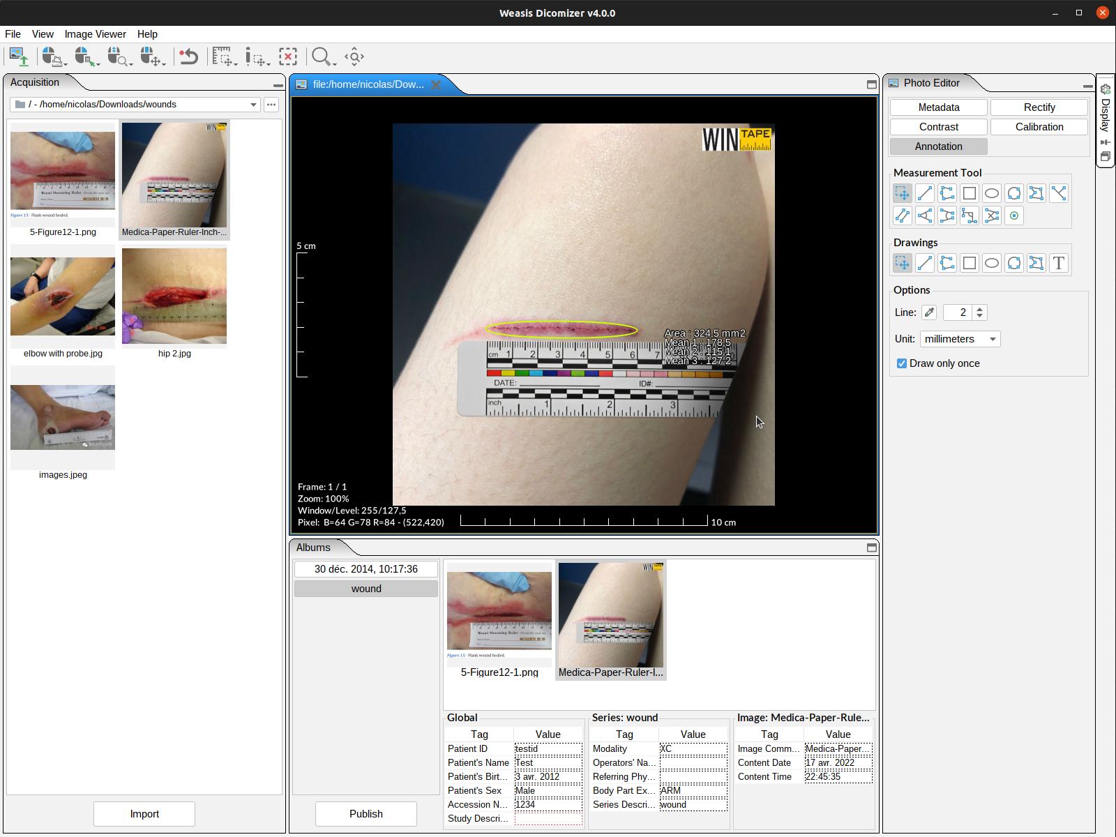
Dicomizer — the workspace for converting standard images into DICOM objects.
Standard image explorer — workspace for non-DICOM images (configured through the non-dicom-explorer.json profile).
DICOM Import
How to import DICOM files
Weasis can ingest DICOM data from many sources:
Drag and drop files, folders, or DICOM ZIP archives from the system file explorer.
Double-click a DICOM file in the system file explorer (file association).
Local Device — browse files, folders, or DICOM ZIP archives from inside Weasis.
DICOMDIR — load a DICOM CD/DVD or any folder that contains a DICOMDIR index.
DICOM Query/Retrieve — query a remote PACS over classic DICOM (C-FIND / C-MOVE / C-GET) or DICOMweb (QIDO / WADO-RS) and retrieve selected studies.
Commands — local or remote commands launching Weasis with a target series (see the Weasis Protocol).
To send data the other way — out of Weasis to a file, a PACS node, or a CD/DVD — see DICOM Export.
Note
Whatever the import method, a popup may appear at the end of an import in any of these cases:
Error — one or more DICOM files cannot be read because they are corrupted or malformed (since Version4.3.0).
Information — since Version4.7.0, one or more valid DICOM files were skipped because their SOP Class has no viewer available (e.g. Raw Data Storage). These files are not corrupted, they are simply not displayable. The notification can be silenced with the Don’t show this again checkbox in the dialog, or from the DICOM Explorer preferences (Notify when DICOM files with an unsupported SOP Class are skipped).
Network error — when a network error occurs during a retrieve (DICOMweb or WADO), a message offers to download the missing files again.
From the system file explorer
Drag and drop
Files, folders, or DICOM ZIP archives selected in the system file explorer can be opened by dragging and dropping them into the central area of Weasis. The accepted drop target depends on the central panel state:
Empty central panel — any file a Weasis viewer can open, including standard images such as TIFF, PNG, and JPEG.
DICOM Explorer or any DICOM viewer (2D, MPR, 3D, SR, AU…) — only DICOM files and DICOM ZIP archives. Weasis opens each series in the most appropriate viewer.
File association
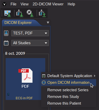
DICOM files can be opened by double-clicking them from the system file explorer.
Note
On Windows, only files with the .dcm extension are associated with Weasis. On other operating systems, DICOM files without an extension are also associated with Weasis.
From the Weasis menu or toolbar
Two import entry points sit next to each other in the toolbar (and under File > Import in the main menu):
The first button opens the standard DICOM import dialog described below (File > Import > DICOM).
The second button is a shortcut for the DICOMDIR / CD-ROM workflow (File > Import > DICOM CD).
Local Device
Since Version4.7.0, DICOM ZIP is also accepted in the local-import workflow:
Files — browse and select one or more DICOM files or DICOM ZIP archives via the file chooser. If a ZIP archive is password-protected, a password prompt is shown.
Folders — browse and select one or more folders via the file chooser. Folders containing DICOM ZIP archives are also supported.
Search recursively — when enabled, the import also descends into subdirectories.
DICOMDIR
Loads a DICOMDIR-based study from a CD/DVD or any folder that already contains a DICOMDIR index file:
Path — browse to a folder containing a DICOMDIR.
Detect CD-ROM — try to load a DICOM CD/DVD directly.
Copy images into the local temporary directory — useful for slow reading devices such as CD-ROM drives.
DICOM Query/Retrieve
Queries a remote PACS and retrieves selected studies into the DICOM Explorer. The dialog has two tabs — DICOM Source and Search Criteria.
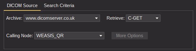
DICOM Source tab
Archive — pick the remote node to query:
DICOM nodes — classic DIMSE (C-FIND for the query, plus C-MOVE, C-GET, or WADO-URI for retrieval).
DICOMweb nodes — QIDO for the query, WADO-RS for the retrieval (no additional options needed).
Retrieve (DICOM archives only) — the protocol used to transfer the images:
C-MOVE — the classic DIMSE retrieve. Accepts all SOP Classes but is not recommended over the web.
C-GET — transfer syntaxes are negotiated per SOP Class through a configuration file.
WADO-URI — C-FIND for the query plus WADO-URI retrieve; requires a WADO server.
Calling Node (DICOM archives only) — pick the calling DICOM node that matches the remote AE.
More options — opens the preferences so you can add or edit DICOM nodes.
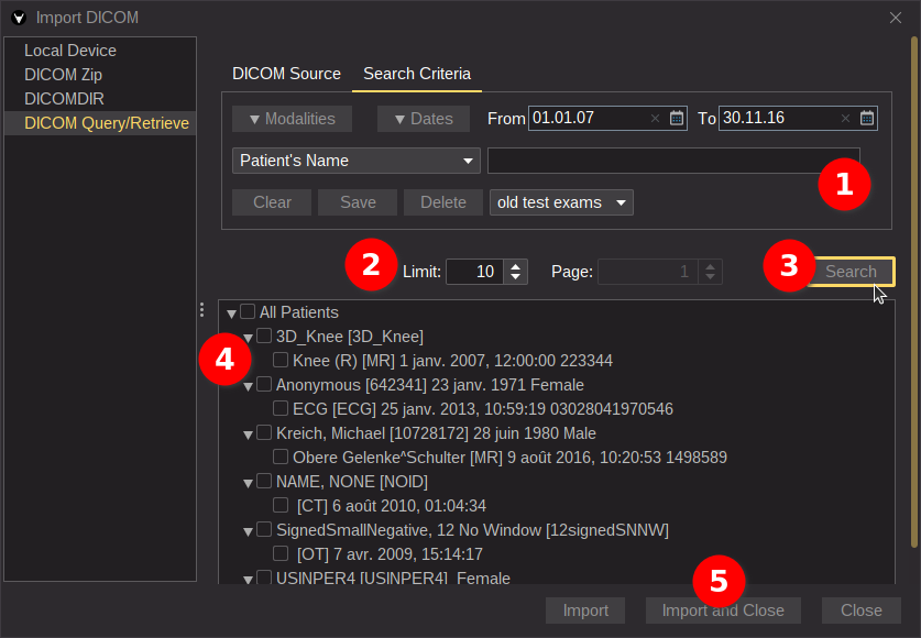
Search Criteria tab
Pick a pre-registered search (combo box at the bottom-right of the Search Criteria panel) or fill in your own criteria. Saved criteria can be reused later; since Version4.1.0, the item selected in the combo box is re-applied automatically the next time the window opens (the default is Empty).
Adjust the limit — the maximum number of studies returned by the query. Set the limit to 0 to remove the cap. For DICOMweb, the limit is the page size; use the spinner buttons to move between pages.
Click Search.
Select the studies you want to import.
Click Import and close the window.
Note
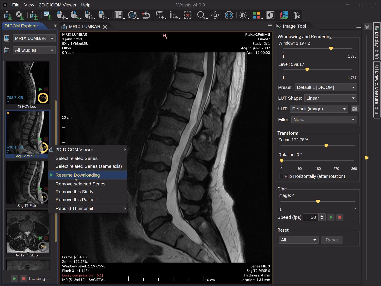
Tracking the download progress and pausing the download of a series is supported only with DICOMweb nodes and with the combination DICOM C-FIND + WADO-URI.
A paused series can be resumed by clicking the green play button or via its right-click menu.
Tip
If a query runs for too long, click Clear in the Search Criteria panel to cancel the request.
When using a DICOMweb node, an external login may be required (for instance signing in to a Google account in your web browser). If the login fails, Weasis can freeze for up to a minute waiting for the authorization code.
From commands
Weasis can be started — or asked to load a specific study — through commands launched locally or remotely. See Examples to load images on the Weasis Protocol page.
DICOMweb Configuration
How to configure a DICOMweb node
DICOMweb is the modern, HTTP-based set of DICOM services (QIDO-RS for query, WADO-RS for retrieve, STOW-RS for store, plus the legacy WADO-URI). Once a DICOMweb node is configured in Weasis, it shows up in the DICOM Query/Retrieve dialog and behaves like any other archive.
This page covers manual configuration inside Weasis. If you embed Weasis in a web portal, you can also launch it from a web context so that the DICOMweb parameters are derived automatically from the launch URL — no per-user configuration required.
General Configuration Steps
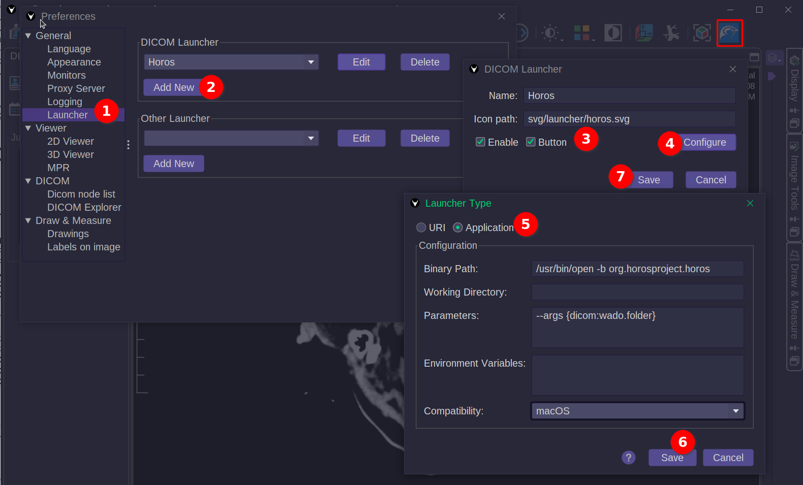
Open File > Preferences (Alt + P).
Select DICOM node list in the left sidebar.
Click Add new to create a new node, or select an existing one and click Edit.
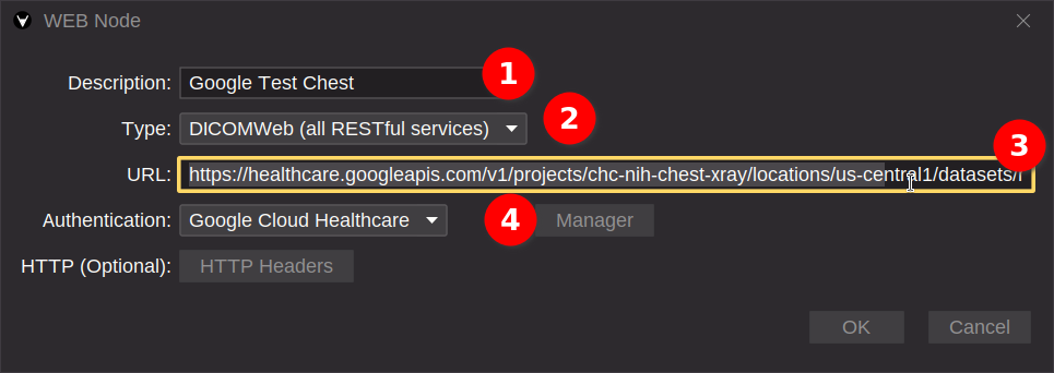
In the node dialog:
Give the node a descriptive name.
Pick a service type. The default DICOMweb (all RESTful services) covers query, retrieve, and store at once. To restrict the node to a specific service, pick one of:
QIDO-RS — query.
STOW-RS — store.
WADO-URI (non-RS) — legacy single-object retrieval. Combines a classic C-FIND query with a WADO-URI retrieve (see Query/Retrieve).
WADO-RS (Retrieve) — modern retrieve.
Enter the service URL of the DICOMweb server.
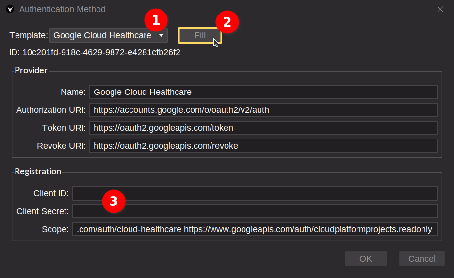
Configure authentication by clicking Manager, then Add:
Either pick a template from the list and click Fill to populate some fields, or fill them in manually.
In the Provider panel, every field is mandatory.
In the Registration panel, every field is optional — except for OAuth2, where the Client ID, Client Secret, and Scope must be filled. Audience is optional, but some providers need it.
The Grant Type selector chooses the OAuth2 flow:
code (Authorization Code, the default) — interactive login: Weasis opens your browser so you sign in with your account, then receives the token through a loopback redirect. Use this for user-facing access.
client_credentials (Client Credentials, RFC 6749 §4.4) — non-interactive, server-to-server: Weasis obtains the token directly from the token endpoint using only the Client ID and Client Secret, with no browser login. Use this for service/headless accounts.
Click OK to save the authentication.
Optionally, add HTTP headers that should be sent with every request to this service URL (useful for tokens or other custom auth schemes).
Click OK to save the node.
Then open the DICOM Import dialog and pick the new node. If OAuth2 is configured with the Authorization Code grant, the first query opens your browser to complete the sign-in; subsequent queries reuse the cached token. With the Client Credentials grant, no browser login is required — Weasis authenticates silently using the configured Client ID and Secret.
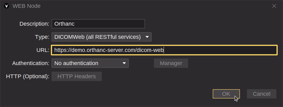
The screenshot below is configured for the public demo server, which requires no authentication. For your own Orthanc instance, replace the URL and configure the authentication method as described in the general steps.
https://demo.orthanc-server.com/dicom-web
Note
The DICOMweb implementation in Orthanc does not currently support the thumbnail service, so series thumbnails will not preview before the full retrieve.
dcm4chee-arc-light
dcm4chee-arc-light is a robust open-source PACS that exposes DICOMweb services out of the box.
To configure a dcm4chee-arc-light node (see also the general steps):
Add a new DICOMweb node.
Enter a description (e.g. DCM4CHEE Archive).
Pick the DICOMweb service.
Enter the URL of your dcm4chee-arc-light server. The default endpoint follows this pattern:
Almost every panel and viewer tab in Weasis can be moved, split, pinned, or hidden by dragging it with the mouse. This lets you arrange the workspace around the task at hand — for instance comparing two series side by side, putting the MPR viewer and the 3D Volume Renderer next to each other for crosshair-driven volume cutting, or maximizing a single view for a focused read — without leaving the application.
Central View
The central area is where viewers and players are displayed as tabs. It supports two main layout operations.
Splitting tabs
Reorganize tabs by dragging and dropping them:
Drag a tab toward an edge (top, bottom, left, or right) of the central area to split the space and display two tabs side by side or stacked.
Drop a tab onto another tab group to merge it back into a single area.
This makes it possible, for example, to compare two series simultaneously in a split-screen layout, or to keep an MPR tab next to a 3D rendering of the same volume.
Tip
To return to a single-tab layout, drag one of the split tab groups back onto the other, or close the extra view.
Maximize a tab
A tab can be maximized to occupy the entire application window, including the space normally taken by the tool panels on either side — giving the largest possible viewing area for a single viewer.
Maximize — click the maximize button in the tab header, or double-click the tab.
Restore — click the normalize button, or double-click the tab again.
Tool Panels
The strips on the right side of the central area host the tools attached to the active viewer (measurements, image adjustments, display options, segmentation, …). Each tool panel can be managed independently with one of three display modes.
Docked
The default mode: the tool panel is docked in the vertical strip next to the central view. In this mode it is always visible and takes up a fixed portion of the screen.
Pinned as overlay
The tool panel floats on top of the central view without reducing the viewer’s size. Useful when you want the maximum viewing area while keeping quick access to the tools.
Click the pin icon in the tool panel header to switch to overlay mode.
The overlay can be repositioned by dragging its title bar.
Minimized (vertical button)
The tool panel collapses to a small vertical button on the side of the interface. Clicking the button temporarily reveals the panel without permanently giving up screen space.
Click the minimize icon in the tool panel header to collapse it to a button.
Click the button again to restore the panel.
Rearranging tool panels
Inside the vertical strip, individual tool panels can be split and re-docked relative to each other:
Drag a tool panel header and drop it above, below, or beside another tool panel to split the tool area and display several tools at once.
Drop a tool panel onto another tool panel’s tab bar to group them as tabs within the same slot.
This lets you arrange the most-used tools exactly where you want them for a given reading workflow.
Note
The docking layout is not currently saved between sessions. Panel positions and splits can depend on the displayed data and on the environment (screen resolution, number of screens), which makes reliable persistent restoration impractical for now.
DICOM Export
How to export DICOM files
Weasis offers two complementary export workflows:
Export the selected view — produces a raster image (PNG, TIFF, JPG, JPEG 2000) or a clipboard copy of what is currently shown on screen. Useful for slides, reports, e-mails, screenshots of measurements, and other non-DICOM consumers.
DICOM Export — produces DICOM-format output (a directory tree, an ISO image, or a network transfer to a remote node). Use this to share studies with another DICOM-capable system without losing pixel fidelity or metadata.
Exporting the selected view
Open the export-view dialog from the toolbar icon
or from the main menu File > Export > Exporting view. The output can be sent to the clipboard or saved to an image file in PNG, TIFF, JPG, or JPEG 2000 format.
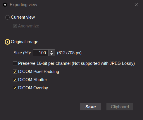
Current view
Exports the view exactly as it appears on screen, at its current size and with every overlay (annotations, measurements, DICOM annotations, rulers…) visible.
Anonymize — removes identifying information from the overlay, in line with the Anonymize option of the 2D viewer.
Original Image
Exports the underlying image — without on-screen overlays — with a few rendering options.
Size — scale the exported image (percentage of the original dimensions).
Preserve 16-bit per channel — keep the original pixel depth (16-bit in PNG / JPEG 2000 / JPEG-XL / TIFF, double values in TIFF). When checked, the exported pixel values match the Modality LUT values (e.g. Hounsfield units for CT). JPEG Lossy is only available with this option unchecked, since the format requires an 8-bit image.
Open the DICOM Export window from the toolbar icon
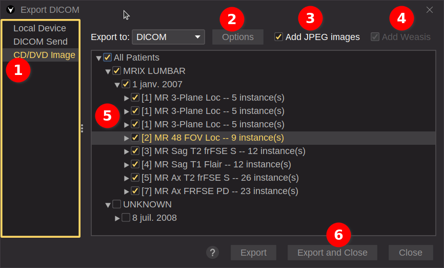
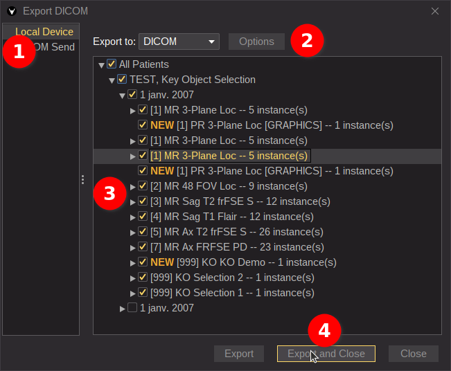
or from the main menu File > Export > DICOM. Three destinations are available in the left panel — Local Device, DICOM Send, and CD/DVD Image — each with its own set of options.
Tip
When the export window opens, the study that was selected in the viewer (orange focus border) is pre-checked, and the series that are currently open are highlighted with a full-line selection.
Hover any series row to see its thumbnail in a tooltip — useful when picking among several similar series.
Local Device
Select Local Device.
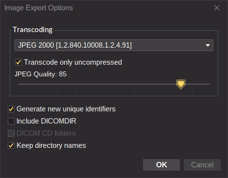
Choose the export options:
Transcoding — change the DICOM transfer syntax (compression / encoding) of the exported files. Leave the default unless you specifically need a different syntax.
Generate new unique identifiers — replace the Study / Series / SOP Instance UIDs with newly generated ones. Cross-references between UIDs are kept consistent within this export session only — running the export a second time produces a different set of UIDs that no longer matches the first.
Include DICOMDIR — write a DICOMDIR index file alongside the exported objects.
DICOM CD folders — wrap the exported tree in the standard DICOMDIR-compliant folder layout used on DICOM CDs.
Keep directory names — preserve human-readable folder names in the exported hierarchy (incompatible with the strict DICOMDIR layout).
Pick the patient(s), study (or studies), series, or individual instances to export. Series created inside Weasis (such as Key Object / Presentation State objects) are marked with a NEW flag.
Click Export to write the files, then close the window.
Note
When the export uses a native image format (JPG, PNG, JPEG 2000, JPEG-XL, or TIFF) instead of DICOM, only the image frames are converted (see the Original Image options). Encapsulated DICOM payloads — video, audio, and PDF — are extracted as standalone files in their native format.
Multi-frame images are exported as numbered files (one frame per file).
DICOM Send
Sends the selected objects directly to a remote DICOM or DICOMweb node over the network — the same protocols used by PACS systems for inter-institutional transfer.
Select DICOM Send.
Choose the destination node — a classic DICOM node (C-STORE) or a DICOMweb node (STOW-RS).
Pick the patient(s) / study / series / instances to send. Series created inside Weasis are marked with a NEW flag.
Click Send to transfer, then close the window.
Tip
Destination nodes are configured under File > Preferences > DICOM (see the DICOM Node List and DICOMweb Node List entries) and can be reused across export sessions.
CD/DVD Image
Produces a burnable ISO image that follows the DICOMDIR layout expected by most CD/DVD-based DICOM media.
Select CD/DVD Image.
Choose the export options:
Transcoding — change the DICOM transfer syntax of the exported files. Leave the default unless you specifically need a different syntax.
Generate new unique identifiers — replace the Study / Series / SOP Instance UIDs with newly generated ones. Cross-references between UIDs are kept consistent within this export session only — running the export a second time produces a different set of UIDs that no longer matches the first.
Add JPEG images — also extract every image and every encapsulated payload (video, audio, PDF) into a separate JPEG folder for easy preview on systems without a DICOM viewer.
Add Weasis — embed the Weasis viewer directly into the ISO so the recipient can launch it from the media. Currently supported only on Windows x86-64 (both for producing and for running the embedded copy). Running Weasis straight off a CD/DVD is slow; for a better experience, write the ISO to a USB stick or open the disc with a locally installed copy of Weasis as described in the README.html on the disc.
Pick the patient(s) / study / series / instances to export.
Click Export to write the ISO, then close the window.
DICOM Explorer
Structure and display of Patients/Studies/Series
DICOM Explorer
The DICOM Explorer is the panel on the left side of the application. It displays everything you have loaded into Weasis as the Patient / Study / Series / Image hierarchy defined by the DICOM standard, and is the starting point for opening a viewer on any series.
Data can be added to the Explorer in several different ways — drag-and-drop, the import dialog, a PACS query, or the Weasis Protocol.
Tip
You can navigate through the Patient / Study / Series / Image structure using only keyboard shortcuts (the bindings below are the defaults — customizable since v4.7.0). For example:
Open an image and, if necessary, select the view to focus on. If the layout has more than one view, you can move across the views with Tab and Shift + Tab. The view surrounded by an orange line is the focused view.
Navigate through images within a series with Up and Down.
Navigate through series within a study with Left and Right.
Navigate through studies within a patient with Ctrl + Left and Ctrl + Right.
Navigate through patients with Ctrl + Up and Ctrl + Down (follow the order in the patient’s combo box and select the last tab if a patient has several tabs already open). To navigate open tabs, use Ctrl + Tab and Ctrl + Shift + Tab.
Patient Level
Weasis can display several patients at the same time. By default, when images are imported, a tab with the patient’s name opens in the main area.
A tab containing a multi-view layout can only display images from a single patient.
You can switch between patients either through the first combobox in the DICOM Explorer (see image above) or by selecting a tab in the main area.
In the combobox, patients are sorted alphabetically — case-insensitive, and according to the active regional setting.
Since Version4.7.1, the patient combobox is searchable — click it and start typing part of a patient name (placeholder Search patient…) to narrow the list to matching patients. To restore the full patient list, click the clear button (✕) on the right of the field, then open the combo to select a patient.
Studies and series are grouped under the same patient when their Patient Name and Patient ID both match. Otherwise, a new patient entry is created.
Study Level
A study contains one or more series (thumbnails) that belong to a single patient. A surrounding line groups the series of one study (see the image above).
Studies are sorted in reverse chronological order by default. Since Version4.1.0 the sort order can be changed in File > Preferences > DICOM > DICOM Explorer under Study data sorting. If a study has no study date, it is sorted alphabetically by Study Description.
All studies are shown by default; the study combobox can restrict the view to a single one.
Series Level
A series is represented by a thumbnail with the image count shown in the bottom-left corner.
Select related Series — right-click a series and choose Select related Series to highlight every series in the study that shares its Frame of Reference UID (the DICOM coordinate system). Open them together (right-click again → 2D Viewer > Open) to get cross-coupled views that auto-synchronize and that the 3D cursor can drive.
Tip
Series built inside Weasis — the MPR viewer (Build a new series from the current view / Build three series from MPR views) and the MIP viewer (Build a new Series) can add reconstructed series back into the Explorer. These newly built series join the current study and can be opened, sent, or exported like any other series.
Filtering the series list
Since Version4.7.1, a search field above the thumbnail list narrows the series shown for the currently selected patient. The small button on the left of the field selects one of three exclusive filter modes — click it to switch (its tooltip reads Filter mode: … (click to change)). A counter next to the field reports how many series pass the filter (shown / total series shown).
Mode
What it does
Full text
Type any text to match the series Description, Modality, Body Part Examined, Protocol Name and Series Number, as well as the parent study’s Description, Study ID and Accession Number. Existing series and study descriptions are suggested as you type.
Study date
Pick a single study — listed by date — to show only its series, or choose All studies to remove the restriction.
Modality
Pick one or more modalities (e.g. CT, MR) from the suggestions to show only the matching series.
Each patient keeps its own filter: switching patients restores the filter last used for that patient. Because only one mode is active at a time, changing the mode clears the current criterion.
To show the full series list again, click the clear button (✕) on the right of the field to reset the search, then open the combo to pick from all entries.
4D Series Sub-Series Splitting
When a DICOM series is loaded, Weasis automatically analyzes it to detect multi-phase acquisitions (e.g. cardiac phases, contrast phases, 4D volumes). If multiple phases are detected, the series is split — automatically or with a confirmation step — into separate sub-series, one per phase. Each sub-series can then be used independently in the MPR, MIP, or 3D Volume Renderer.
Splitting behavior by number of detected phases
Phases
Behavior
1
No split — treated as a standard single-phase series.
2 – 7
Automatic split — the series is immediately divided into one sub-series per phase, without any user interaction.
≥ 8
Manual split — Weasis stores the phase count but leaves the series intact. A confirmation dialog is shown before splitting to prevent unintended fragmentation of large datasets.
Manual split confirmation dialog (≥ 8 phases)
When 8 or more phases are detected, a dialog asks you to confirm the split. Once confirmed, the series is divided exactly as in the automatic case. Canceling leaves the series intact as a single entry in the DICOM Explorer.
Sub-series structure after splitting
After splitting, each phase becomes a separate thumbnail in the DICOM Explorer. The first sub-series reuses the original series entry; the additional sub-series are added to the study tree, identified by a # number in the upper-right corner of the thumbnail.
Tip
Open any individual phase sub-series in the MPR, MIP, or 3D viewer for accurate volumetric analysis — each sub-series contains only the images of a single phase and can be reconstructed as a coherent 3D volume.
If the split is not needed, or was triggered unintentionally, the sub-series can be merged back. Select the thumbnails you want to merge (all or a subset) and choose Merge Selected Series from the context menu — the selected sub-series are recombined into a single series entry.
Note
Phase detection is based on the spatial position of each image. If multiple images share the same slice position, they are assumed to belong to different temporal phases. If no such overlap is found, the series is treated as a standard single-phase acquisition and is never split.
Series Display and Opening
By default, series are sorted by series number; if that is missing, they are sorted chronologically by series date or another available date.
To open a series:
Drag and drop a thumbnail into the main area. If the drop lands in a view of the same patient, that view’s series is replaced; otherwise, a new tab is created.
Double-click a thumbnail (or navigate with the Up / Down arrows and press Return). If a view of the same patient already exists, the series in the focused view (orange border) is replaced.
Select one or more thumbnails and pick an action from the 2D DICOM Viewer context menu:
Open — opens the series in the most appropriate layout (replaces the series if a patient tab already exists).
Open in new tab — same, but always in a new tab.
Open in screen — same, but on a specific screen.
Add — appends the series to the current patient’s layout, if one exists.
Note
Since Version4.7.0, tab opening and focus behavior is handled automatically, replacing the old configurable opening mode preference.
When is a new tab opened?
A new viewer tab is opened for every patient whose studies are loaded via an import action. If the patient already has an open tab, the new studies are added to that existing tab instead of opening a new one. This keeps each patient organized in a single tab and prevents fragmentation of the workspace.
How is focus managed?
Focus follows an automatic policy based on loading duration:
If the study finishes loading quickly (within ~3 seconds), the new tab comes to the foreground — the expected behavior for a direct open action.
If the study is still loading when the threshold is exceeded (for example a slow network import in the background), the current tab keeps focus — Weasis will not interrupt your work by stealing focus for a slow background load.
In practice: fast loads surface immediately, slow background loads stay out of the way.
Preferences
From the main menu File > Preferences > DICOM > DICOM Explorer:
Thumbnail size — width of the thumbnails; the panel adjusts accordingly. Default: 144. Restart the application after changing this value.
Study data sorting — sorts studies in reverse chronological order (default) or chronological order. Since Version4.1.0.
Download all series immediately — when checked, series start downloading as soon as they are queued via WADO or WADO-RS. When unchecked, you must click the play button on each series, or the global play button at the bottom of the thumbnail list. Default: checked.
DICOM 2D Viewer
Displaying DICOM images
The 2D viewer is the default viewer for any DICOM series that contains images — CT, MR, US, CR / DX, mammography, color photographs, and so on. It handles both single images and stacks (volumetric series), and is the entry point for the more specialized viewers such as MPR, the 3D Volume Renderer, and the MIP projection. It can also overlay a PET or SPECT series on a CT/MR base — see Image Fusion.
Open the 2D viewer
The viewer can be opened with
in the toolbar, or by double-clicking a thumbnail (or right-clicking it and choosing 2D Viewer > Open) in the DICOM Explorer.
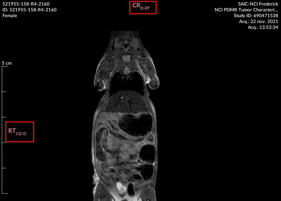
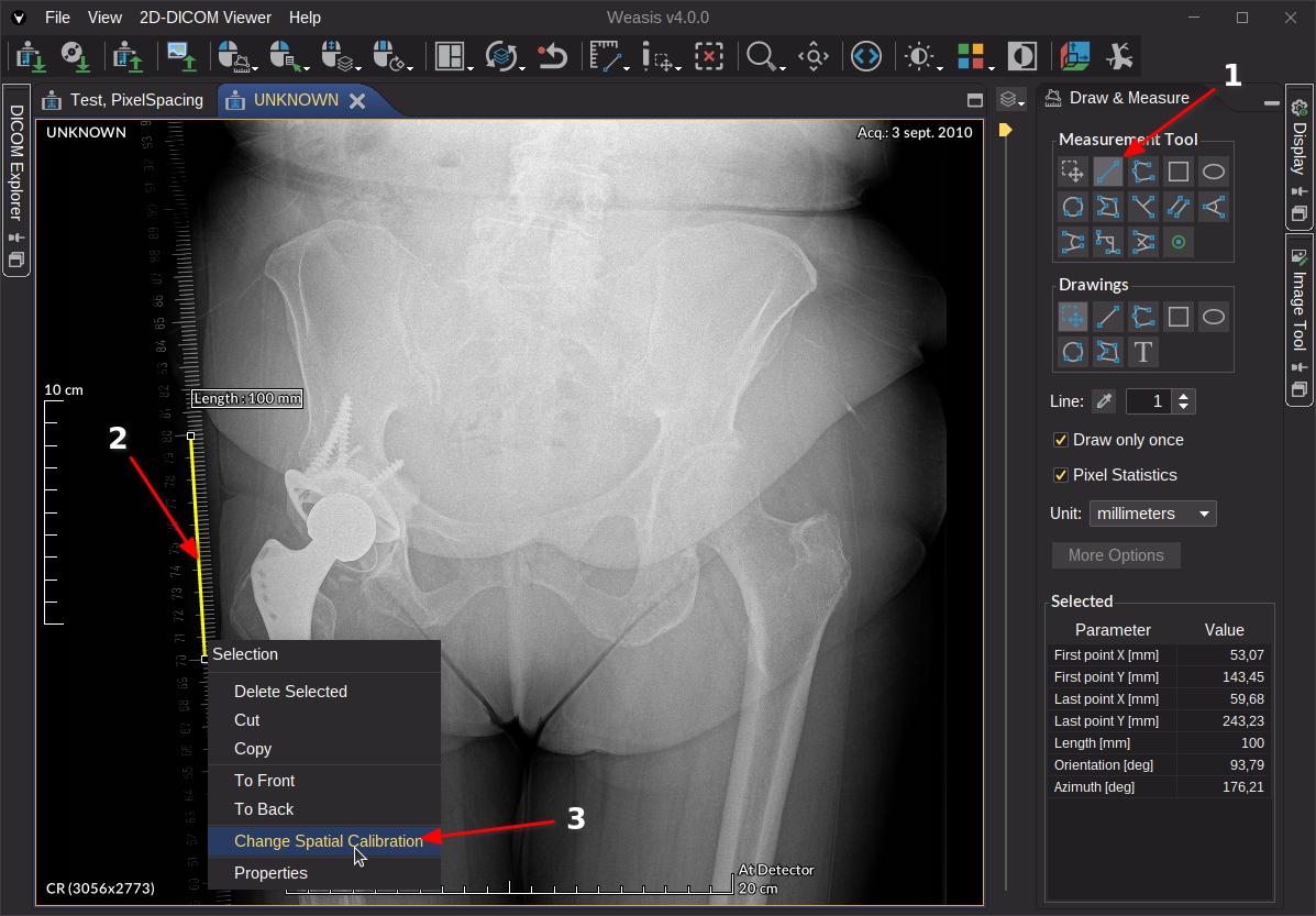
The rulers K display a real-world size whenever Weasis can derive one from the DICOM file. When a small label M is shown above the calibration, it indicates how that calibration was obtained:
At detector: projection radiography calibration taken at the detector plane.
Magnified: projection radiography calibration corrected by the magnification factor (e.g. mammography, as in the screenshot above).
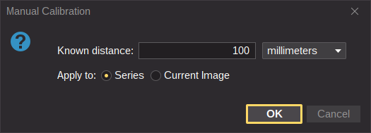
Used fiducials: calibration derived from fiducials (e.g. a manually placed ruler in the image).
At scanner: calibration taken from a digitized medium (e.g. film digitizer).
Toolbars A
Viewer Main Bar
Choose the action assigned to each of the three mouse buttons and the mouse wheel. Defaults are:
Left button — Window / Level. Can also be changed from the context menu F or the keyboard shortcuts.
Right button — Context Menu.
Wheel — Series Scroll.
Middle button — Pan.
Available actions:
Pan — move the image position. T key to select. Alt + Arrows to pan while another action is selected.
Window / Level — change image contrast. W key to select.
Series Scroll — navigate through the images of the current series. S key to select.
Rotation — rotate the image by a free angle. R key to select.
Measure — draw a graphic to measure something. M key to select.
Draw — draw a graphic to annotate. G key to select.
Context Menu — open the context menu. Q key to select.
Crosshair — 3D cursor. H key to select. Ctrl + click or Ctrl + Shift + click adjusts Window / Level without leaving crosshair mode.
No Action — do nothing. N key to select.
Tip
While dragging, hold Ctrl to accelerate the action and Ctrl + Shift to accelerate more.
The single-key shortcuts above are the defaults — most are customizable since v4.7.0 in Preferences > General > Keyboard Shortcuts. See Keyboard Shortcuts.
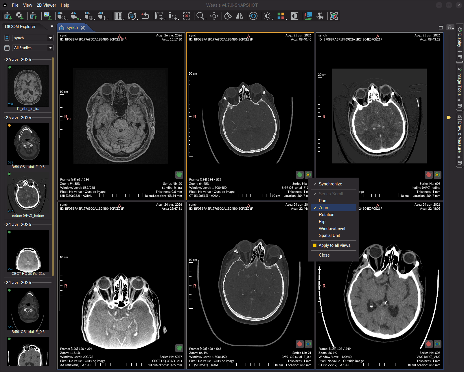
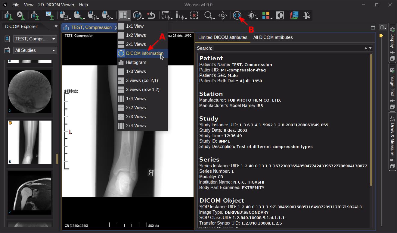
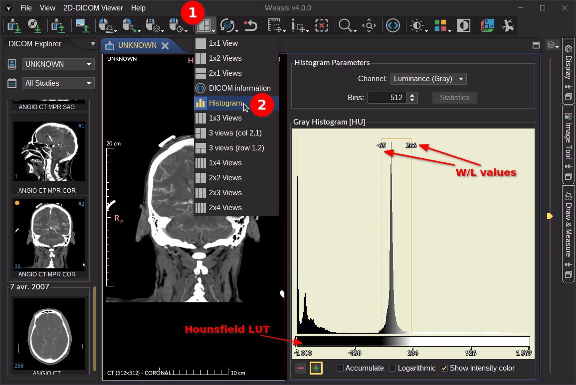
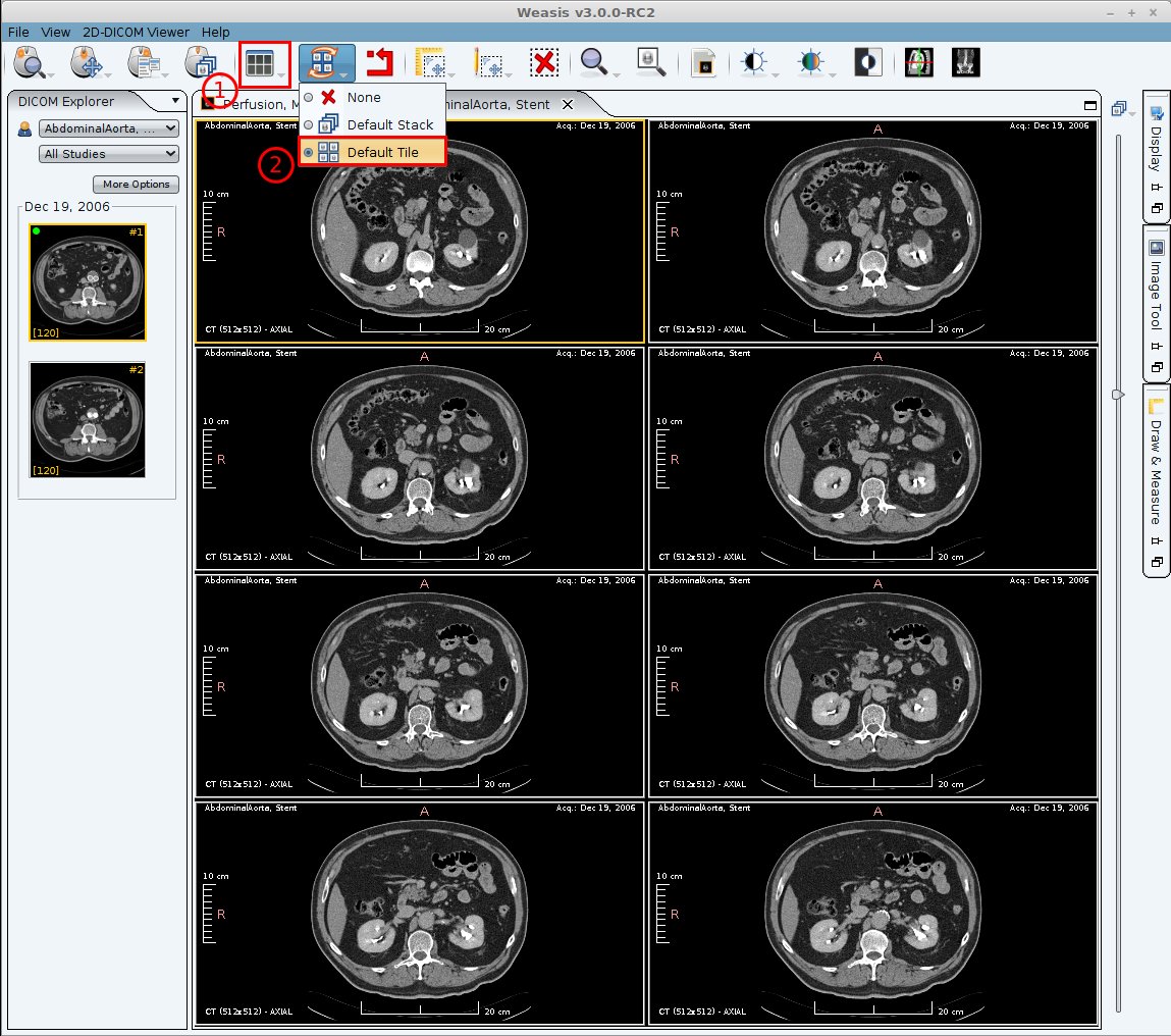
Default layout — change the layout of the view. DICOM Information and Histogram are special layouts that update automatically as you scroll through the series.
Synchronize — apply the same settings (window/level, scroll, zoom, …) to multiple views simultaneously. Two modes are available: Default Stack (the default — couples series sharing the same Frame of Reference UID) and Default Tile (mosaic display of a single series). A master Synchronize checkbox at the top of the drop-down turns synchronization on or off globally without changing the active mode. Each 2D view also exposes its own auto-sync
and manual-sync
overlay buttons in its bottom-right corner. See View Synchronization for the full mechanics, the per-view controls, and the FoR color-chip system.
Reset — restore the default image rendering (see Reset). Escape key to select.
Toolbars can be shown or hidden from the View top menu.
Viewer tools
The right-side panel groups all the tools tied to the 2D viewer.
The mini-tool is always visible; the other panels open by clicking the corresponding vertical button. The normalize button
docks a panel into the main layout — otherwise it opens as a pop-up that can be kept in front with the pin button
(not recommended, as a pinned pop-up hides other panels).
Mini-tool B
By default the mini-tool scrolls through the images of the selected series (the one surrounded by the orange focus border). The combobox at the top can switch it to control zoom or rotation instead.
Display C
Controls how the image and graphic objects are displayed in the view.
The Apply to all views option propagates the chosen display settings to every view in the selected tab. When unchecked, settings apply only to the focused view (orange border).
Image
Display options for the image itself. Unchecking Image hides the image and leaves only the annotations and graphic objects visible. The other options expose DICOM-specific behavior:
Display transformation values and DICOM information directly on the image.
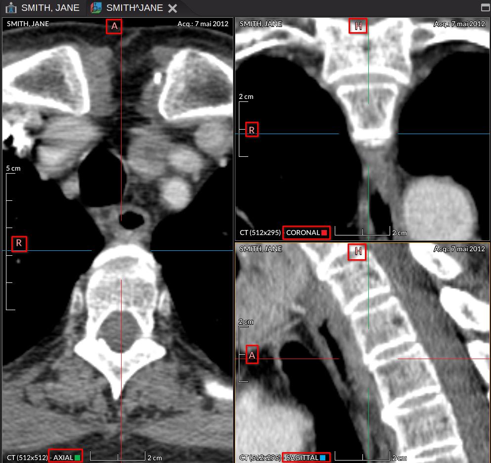
Annotations — DICOM information shown in the image corners:
G Top left — patient information.
H Top right — study information.
I Bottom right — series information (depends on the modality).
J Bottom left — image information and the position of the image in the series.
Minimal Annotations — reduce the number of annotations shown. Press Space or I to cycle through the three states (minimal, none, all).
Anonymize — hide identifying information only inside the views (not in other parts of the GUI such as the tab title). Combine with the screenshot tool when exporting an image.
Scale — display the rulers on the left and bottom of the image K.
Pixel (Value / Position) — display the pixel value and the cursor position J.
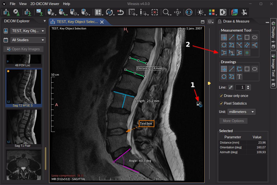
Drawings
Check / uncheck to show or hide the graphic objects (see Draw & Measure).
Image Tools D
Image Tools groups every control that affects how the image is rendered.
Each section below can be collapsed or expanded by clicking its header (since Version4.7.1). The expanded/collapsed state of every section is remembered and restored the next time you open Weasis.
Zoom, rotate, and flip the image. Zoom and rotation can also be driven from the mini-tool or the mouse actions.
Cine
The Cine start button
plays the series at a fixed speed (frames per second). The default speed is taken from the DICOM file when present. Cine options are also accessible from the context menu.
Click Cine stop
to end the animation.
Click the Loop / Sweep toggle
to switch between looping and sweeping playback.
Note
When cine is active, every series currently synchronized with the playing series is animated too. Selecting another series keeps the cine running on it until the Cine stop button is pressed.
For series with a variable frame rate, the playback speed is adjusted automatically, so a value entered manually is not preserved.
Tip
A dedicated Cine toolbar is also available — hidden by default; enable it from the View menu.
Fusion
Overlay a PET or SPECT series on the displayed CT / MR base, with adjustable color LUT and base/overlay opacity (since Version4.7.1). Collapsed by default and enabled only when the study contains a compatible overlay. See Image Fusion for the full workflow, SUV statistics, and MPR inheritance.
Reset
Returns the image to its default rendering, either for every parameter or for a specific one. Also available from the toolbar button
and from the context menu.
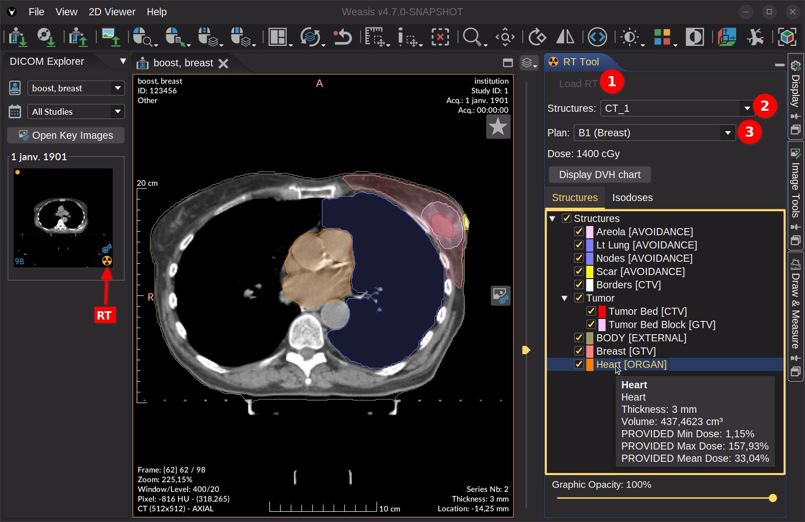
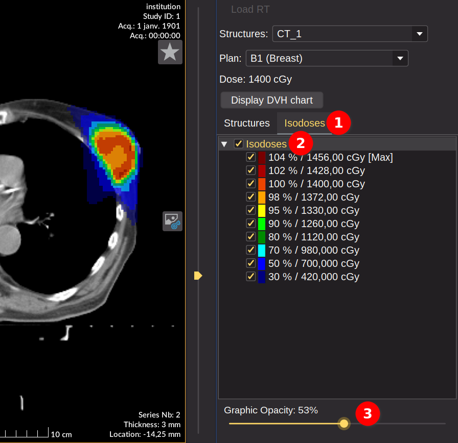
DICOM RT tools — for radiotherapy studies (RTSTRUCT, RTPLAN, RTDOSE).
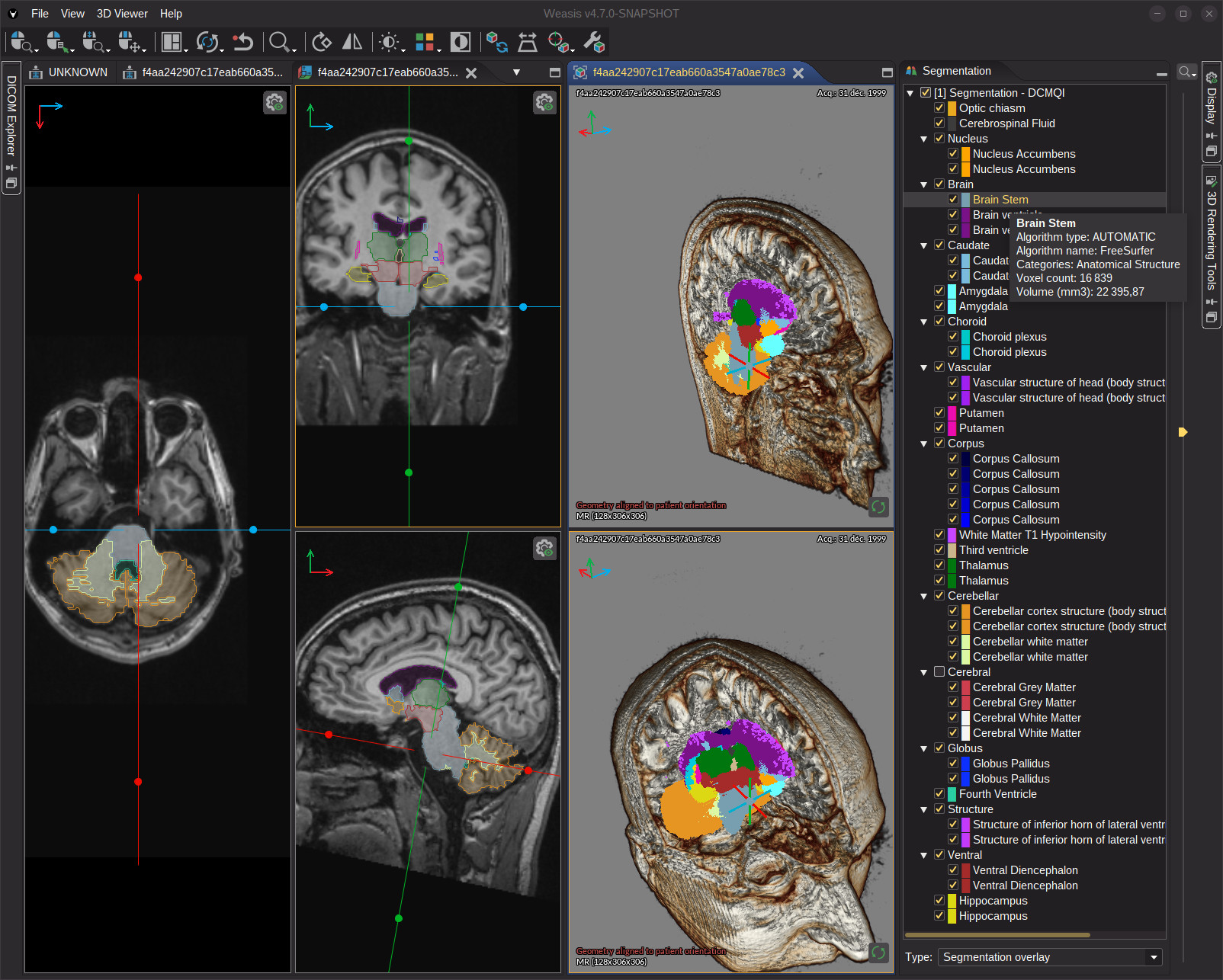
DICOM Segmentation — for pixel-based SEG overlays (binary, fractional, label-map).
Preferences
From the menu File > Preferences > Viewer > 2D Viewer.
Mouse Action Sensitivity
Adjust how strongly a mouse drag translates into action for: Window, Level, Zoom, Rotation, and Series Scroll.
Zoom
Zoom interpolation controls how new pixels are computed when the image is zoomed in or out:
Nearest neighbor — the simplest method: extends the nearest pixel value as-is.
Bilinear — averages the four neighboring pixels. Slightly sharper than nearest neighbor, slightly slower.
Bicubic — uses a 16-point kernel. Sharper than bilinear, but the slowest of the four.
Lanczos — uses a sinc kernel; produces the sharpest results, with performance between bilinear and bicubic.
The default is Bilinear. Nearest neighbor is the fastest option but produces aliasing artifacts.
Other
Apply Window / Level on color images — when checked, the window / level is applied to the RGB channels. Unchecked, window / level has no effect on color images.
Inverse level direction — when checked, the level direction with mouse drag is inverted (dragging down increases brightness), matching the Basic Image Review profile. Unchecked, dragging down decreases brightness.
Apply by default the most recent Presentation State — when checked, the most recent Presentation State object is applied automatically. Otherwise it has to be selected manually via
.
Overlay color — color and opacity of the DICOM overlay. The default is white; the opacity is the transparency / alpha slider of the color picker.
View Synchronization
Synchronizing Views
View synchronization propagates the same actions (scroll, zoom, window / level, …) across several views at once. Weasis offers two synchronization modes — an automatic mode driven by shared DICOM geometry (the Frame of Reference UID, abbreviated FoR throughout this page) and a manual mode to bridge views that the automatic mode cannot connect (only for scrolling).
Frame of Reference: the shared coordinate system
Two series carry the same Frame of Reference UID (DICOM tag 0020,0052) when they were acquired in the same 3D coordinate system. In practice, sharing the same Frame of Reference means sharing the same 3D coordinate system: every voxel in those series is positioned against the same origin and the same axes, so the point at coordinates (x, y, z) refers to the exact same physical location in all of them.
Acquisitions performed in the same session without moving the patient typically share a Frame of Reference, for example:
the CT and the PET produced together by a hybrid PET / CT scanner,
all the slices of a single MR sequence,
a planning CT and the RTSTRUCT / RTPLAN / RTDOSE objects derived from it.
This shared geometry is what makes automatic synchronization possible: when Weasis sees the same FoR on two views, it can align them in 3D without any manual configuration. Series acquired in separate sessions, on different scanners, or after the patient has moved typically have different Frames of Reference and must be coupled with manual sync instead.
The Frame of Reference is the linking concept used by:
Auto-synchronization (see Default Stack Mode below) — propagates scroll, zoom, window/level, … between views sharing a FoR.
The 3D cursor (crosshair) — clicks on one view jump to the same anatomical point in every other view sharing the same FoR.
The MPR viewer — the three reconstruction planes are always FoR-coupled by the crosshair.
Synchronization Modes
The synchronization mode is controlled by the drop-down button
next to the layout button
in the toolbar.
Mode
Description
Default Stack
Couples views from different series that share the same Frame of Reference UID. Scroll only is propagated by default; every other per-action toggle (Pan, Zoom, W/L, Rotation, Flip, …) is opt-in. This is the default mode.
Default Tile
Lays out consecutive images of the same series in a mosaic (n, n+1, n+2, …). Every per-action setting is propagated by default so the whole tile group behaves as a single coherent display.
The drop-down popup also contains:
A non-interactive series-name header at the top of the popup, identifying the currently selected view. It makes explicit that the per-action toggles and the Apply to all views entry below reflect this specific view’s synchronization options.
A master Synchronize checkbox — a global switch that turns synchronization on or off for the whole synchronization session (every participating view, including auto-synced views in other linked containers) without changing the active mode. This is broader than the per-view
button, which toggles only the single view it sits on. Unchecking it makes every view fully independent. See Synchronization scope for how the scopes interact.
An Apply to all views entry — decorated with the selected view’s FoR color chip — that propagates the configuration to every other sync-active view in the container, regardless of FoR (broader than the same-named entry in the per-view popup, which is restricted to the selected view’s FoR group). See Per-view sync controls for the per-action semantics and the color-chip system.
Note
The synchronization mode can also be set programmatically with the command:
dcmview2d:synch VALUE
where VALUE is Stack or Tile. See Commands for details.
Synchronization Scope
Synchronization operates at three different scopes. Knowing which is which avoids surprises when more than one viewer window is open:
Global (whole session) — the master Synchronize checkbox in the toolbar drop-down is a global switch: it enables or disables synchronization for every participating view at once, not just the selected view.
Across containers (auto-sync) — Default Stack auto-synchronization is not limited to a single container. Views in any other visible container that belongs to the same group (the windows opened together from one patient/study group) and is also in Stack mode are kept in sync as well. Open the same study in two windows and scroll, Window / Level, etc. stay coupled across both.
Within one container (manual sync) — manual sync only links views that live in the same container window; you cannot manually link a view to one in another container. In addition, only one manual-sync session can be active at a time across the whole application — starting manual sync on another eligible view joins the existing session rather than creating a second, independent group.
Default Stack Mode (Auto Synchronization)
Default Stack is the most common synchronization mode. When two or more series share the same Frame of Reference UID, Weasis can synchronize their views automatically.
By default, only Scroll is propagated — navigating to a slice in one view moves the other views to the closest matching anatomical position. Every other action (Pan, Zoom, Rotation, Flip, Window / Level, Spatial unit) starts disabled, and you opt them in explicitly through the per-action toggles in either:
the toolbar drop-down popup (applies to the selected view; use Apply to all views to propagate the change to its FoR group), or
the per-view auto-sync popup opened from the
button on the view itself.
Typical use case: display a CT series and its corresponding PET series side by side. Because both series share the same Frame of Reference UID, scrolling through slices in the CT view automatically scrolls the PET view to the matching anatomical level. To couple Window / Level or Zoom too, enable the action on every view in the group (an action is synced only between views that both have it enabled) — toggle it on one view and use Apply to all views.
Tip
To find which series share the same Frame of Reference, right-click a thumbnail in the DICOM Explorer and choose Select related Series, then open all the selected series together in the 2D viewer.
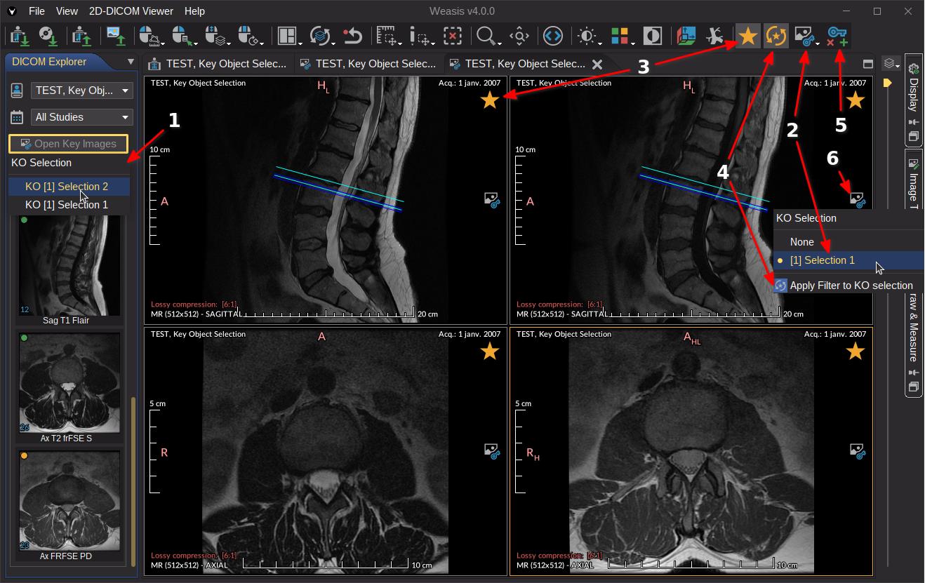
The screenshot illustrates how Weasis advertises synchronization groups visually inside a single layout:
The two views in the left column carry no Frame of Reference UID. Because they are not eligible for auto-sync, the auto-sync
button is not shown on them at all — only the manual-sync
button is available.
The four views on the right form two pairs sharing a Frame of Reference UID, each pair tagged with its own auto-sync color chip: yellow for the top pair, blue for the bottom pair. Auto-sync is propagated only within a same-colored group.
A manual-sync link (hand icon, in green when active) couples one of the FoR-less left views to two peers at once — the other FoR-less view and a view that belongs to one of the FoR pairs — illustrating that manual sync is the fallback to bridge views that auto-sync cannot connect, regardless of whether the peer has a FoR or not.
Per-view Sync Controls
In addition to the global toolbar drop-down, each 2D view carries small overlay buttons in the bottom-right corner that drive its sync behavior independently. They appear whenever the view has at least one eligible peer for synchronization.
Auto-sync button
The
button toggles Default Stack auto-synchronization for this view only. Its appearance encodes two pieces of information:
Outer tint — red when auto-sync is OFF for the view, green when ON.
Center color chip — a small colored square shown when the container holds two or more views with different Frame of Reference UIDs. The color identifies the FoR group; views sharing the same UID share the same chip color, so groupings are visible at a glance. When the container has only one FoR (nothing to disambiguate), the chip is hidden.
Clicking the button opens a per-view sync popup with:
Synchronize this view — master on/off toggle for auto-sync on this view (closes the popup on click).
Per-action toggles — independent checkboxes for Scroll, Pan, Zoom, Rotation, Flip, Window / Level, and Spatial unit. The popup stays open while you flip several options, so you can configure the whole set in one pass.
Apply to all views — copies this view’s effective sync options to every other view sharing the same Frame of Reference UID. The item is decorated with the view’s FoR color chip, matching the chip drawn on the auto-sync button so you can confirm at a glance which group will be affected.
Close — explicit dismiss (the per-action toggles do not auto-close on click; Esc and clicks outside also dismiss the popup as usual).
Note
A per-action toggle only declares whether this view takes part in syncing that action. An action is propagated between two views only when both of them have it enabled — sharing the same Frame of Reference UID is not enough on its own. Enabling Zoom on a single view therefore has no visible effect until at least one peer also has Zoom enabled. To couple an action across a whole FoR group in one step, enable it on one view and use Apply to all views.
Manual sync button
Some series cannot be auto-synced because they have no — or a different — Frame of Reference UID (typical for unrelated CT scans, or legacy series with missing DICOM geometry). The manual-sync button
(same bottom-right corner) lets you link such a view to a peer by relative slice index instead of 3D position.
A view is an eligible candidate for manual sync with the current view when it lives in the same container, has the same orientation, and a different (or absent) FoR — manual sync never crosses containers, and only one manual-sync session can be active across the whole application (see Synchronization scope). Clicking the
button on a view that is currently OFF picks the link target according to how many candidates exist:
A manual-sync group already exists in the container — the new view joins it directly (bidirectional links are added to every member). No picker is shown.
Exactly one candidate — the link is established immediately, no picker.
Multiple candidates and no existing group — a multi-select picker opens so you can pick the views to sync with.
Once active:
Scroll propagation is forced on and locked in the per-view sync popup — manual sync is built on top of scroll. All other per-action toggles (Pan, Zoom, W / L, …) remain freely configurable.
The manual-sync button turns green to indicate that a manual link is established. Clicking it again removes this view from the group.
Tip
The auto-sync
and manual-sync
buttons coexist on the same view. Auto-sync is preferred whenever a shared FoR is available; manual sync is the fallback for views that fall outside any spatial group.
Default Tile Mode
Default Tile mode fills all views in the current layout with consecutive images from the same series. It is useful for reviewing a series at a glance, comparing adjacent slices, or preparing a print layout with multiple images per page.
When this mode is active:
Each view shows a different image of the same series (n, n+1, n+2, …).
Scroll advances the entire tile group by one image at a time.
Every other per-action setting is enabled by default, both user-toggleable (Pan, Zoom, Rotation, Flip, Window / Level, Spatial unit) and always-on internal (Preset, LUT, LUT shape, Invert LUT, Filter, Inverse stack, Sort stack), so the tile group behaves as a single coherent display.
Use the per-action toggles to disable any user-toggleable setting if you want tiles to diverge (e.g. independent zoom for cropped previews).
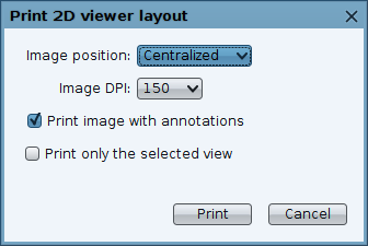
Typical use case: print or export a multi-image layout where each cell shows a different slice of the same series. See Print for more details.
Note
This is the opposite default from Default Stack, where only Scroll propagates and every other action starts off. Tile mode assumes you want everything in lock-step (same series, multi-cell view); Stack mode assumes you want surgical control (different series, cross-modality comparison).
3D Cursor Synchronization
The
3D cursor (crosshair) is a dedicated synchronization mechanism that links the cursor position in 3D space across views that share the same Frame of Reference UID.
Unlike stack mode, which only aligns views near the same anatomical depth, the crosshair lets you click precisely in one view and see that exact 3D point highlighted in every other view simultaneously — regardless of slice or plane orientation.
Two distinct couplings are at play in the MPR viewer:
Internal — between the three MPR planes (axial, coronal, sagittal): these are always cross-synchronized by the crosshair. Beyond that structural coupling, the MPR viewer uses different per-action defaults from the 2D viewer: Scroll, Zoom, and Window / Level are ON by default. The remaining per-action propagations (Pan, Rotation, Flip, Spatial unit) are off by default and can be enabled explicitly.
External — between MPR and other 2D views sharing the same Frame of Reference: the standard Default Stack rules apply (Scroll on by default; every other action opt-in via the per-view toggles described below).
In both cases, the per-view toggles are reached through the Synchronize submenu of each MPR view’s settings popup (see below) — the crosshair coupling itself cannot be disabled.
Per-view sync options in the MPR
MPR views do not show the auto-sync / manual-sync overlay buttons described in Per-view sync controls — synchronization between MPR planes is structural (driven by the crosshair) and cannot be turned off per view. Instead, the per-view sync configuration is reached through a Synchronize submenu in the MPR configuration popup (settings icon
in the top-right corner of the view — listed alongside the other MPR settings).
The submenu is the same as the one opened by the auto-sync button on a regular 2D view, minus the master “Synchronize” toggle (you cannot disable synchronization for a single MPR plane — see above). It contains:
Per-action toggles for Scroll, Pan, Zoom, Rotation, Flip, Window / Level, and Spatial unit. The submenu stays open while you flip several options.
Apply to all views — propagates the current selection to every other view sharing the same Frame of Reference UID. Decorated with the FoR color chip identifying the target group.
Close — closes the popup.
Note
When manual synchronization is active on the view, Scroll is forced on and locked — manual sync is built on top of scroll propagation.
Cine and Synchronization
When the cine animation is active on a series, every series currently synchronized with it (via Default Stack or Default Tile) is animated as well. Cine remains active across series until the Cine stop button
is clicked.
3D Cursor
3D cursor (crosshair)
The 3D cursor — also called the crosshair — lets you click a point on one image and instantly see the same anatomical point in every other view that shares the same 3D coordinate system. Use it to:
Localize a finding on one modality (for example a CT lesion) on the matching PET, MR, or follow-up acquisition.
Cross-check structures between axial, coronal, sagittal and oblique planes.
Compare the same anatomical level on prior and current studies opened side by side.
Two views are linked by the crosshair when they share the same Frame of Reference UID — DICOM’s way of declaring that those series live in the same 3D coordinate system. See Frame of Reference: the shared coordinate system for the full explanation and the typical cases where it applies. Weasis discovers the link automatically from the DICOM metadata — no manual configuration is needed.
Opening related series together
The fastest way to load several series that share a coordinate system:
In the DICOM Explorer, right-click a series and choose Select related Series. Weasis selects every series in the study that shares the same Frame of Reference UID.
Right-click the selection again and choose 2D Viewer > Open to display them side by side.
Activating the crosshair
Select the crosshair
as the active mouse-button action either from the toolbar mouse-button menus or from any view’s right-click context menu. Once active, left-click anywhere in a view and the marker jumps to the matching 3D point in every linked view simultaneously.
Tip
You don’t have to leave crosshair mode to adjust the image: hold Ctrl while dragging to change Window / Level without switching tools. See keyboard shortcuts for the full list of modifiers (most are customizable since v4.7.0).
The crosshair is the position-coupling part of a broader synchronization system. For action coupling (Scroll, Pan, Zoom, Window / Level…) between views sharing a Frame of Reference, see View Synchronization.
Info
For the conventions used to label anatomical directions in multiplanar views, see MPR orientation.
Preferences
The 3D cursor shares two display preferences with the MPR viewer:
Auto-center axes — recenter the views on the clicked point.
Crosshair gap at the center — width of the blank gap around the click point, so the marker does not occlude the structure being inspected.
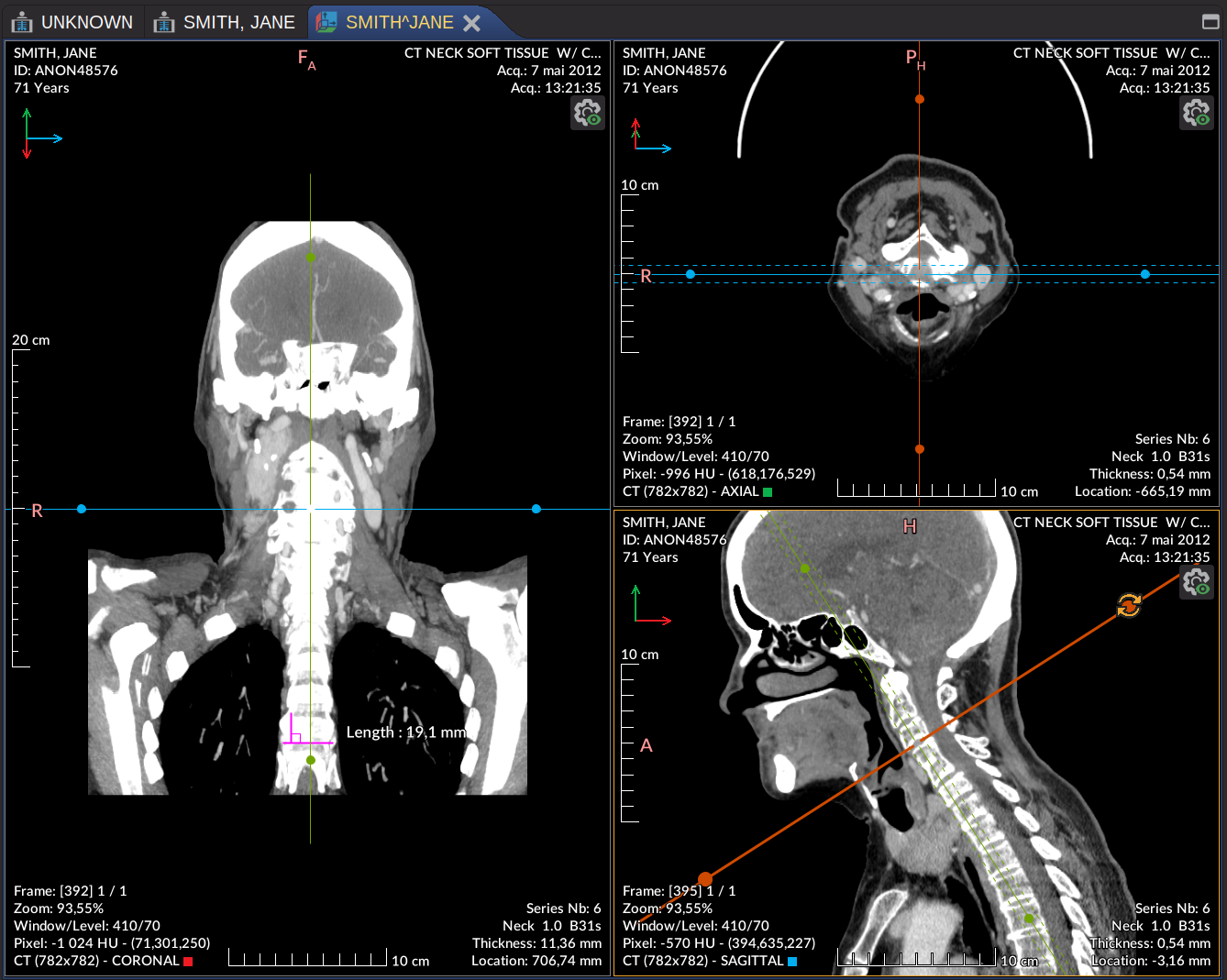
The MPR viewer reconstructs the two complementary anatomical planes from a volumetric acquisition: starting from the original plane (typically axial), Weasis computes the corresponding coronal and sagittal views, all kept in sync through a shared 3D crosshair. Oblique planes are also supported, since Version4.6.0.
The MPR view inherits most of the properties and actions of the DICOM 2D viewer, with one structural difference: the crosshair tool stays active regardless of which mouse action is selected. Open the MPR viewer from the
icon in the toolbar, or by right-clicking a thumbnail in the DICOM Explorer.
Note
The menu and toolbar entries are only enabled when the series contains at least 5 images.
Tip
Opening MPR from a fused 2D view (PET/CT) carries the overlay over to the three planes — see Fusion in the MPR viewer.
Tip
If the series is a multi-phase 4D acquisition (e.g. a cardiac CT with several temporal phases), Weasis automatically splits it into individual phase sub-series when 2–7 phases are detected. For series with 8 or more phases, a confirmation dialog is shown first. Open any resulting phase sub-series to reconstruct it in the MPR viewer — see 4D Series Sub-Series Splitting.
Note
To reconstruct the volume along a curve instead of a flat plane — for example a dental panoramic from a CBCT — draw a polyline and use the Curved MPR actions. See Curved MPR Viewer.
Crosshair actions
The crosshair stays synchronized across the three MPR planes (and with any other FoR-coupled view). Three actions are available on its handles:
Move — translate the cursor in 3D space by dragging the center of the crosshair.
Move axis — slide the crosshair along one axis by selecting and dragging that line.
Rotate — rotate the crosshair around its center by dragging one of the end points along the axes.
Synchronization between MPR planes
The MPR viewer uses different sync defaults from the 2D viewer: in addition to the structural crosshair coupling, Scroll, Zoom, and Window / Level are ON by default between the three planes. The remaining per-action propagations (Pan, Rotation, Flip, Spatial unit) are off by default and can be enabled explicitly. The options live in two places:
The global Synchronize drop-down popup
(next to the layout button) — master on/off plus per-action toggles for the whole container.
The Synchronize submenu in each MPR view’s settings popup — for per-view fine-tuning.
The MPR views can be reorganized into different layouts via the
layout button.
View settings
Open the per-view settings popup with the
icon in the top-right corner of any MPR view:
Center — recenter the crosshair in the view.
Show Center of Crosshair — show or hide the center point.
Show Crosshair — show or hide the crosshair lines. When hidden, the crosshair actions are inactive.
MIP Thickness — slab thickness for the active MIP projection, expressed in slices in the cross-axis direction. Can also be adjusted with Alt + mouse scroll on an axis. Note: the projection may take a moment to refresh, since MIP in MPR is computed in the background and does not use 3D acceleration.
MIP Type — projection mode applied to the slab:
None — no MIP applied.
Min — Minimum intensity projection.
Mean — Mean intensity projection.
Max — Maximum intensity projection.
Build a new series from the current view / Build three series from MPR views — save the reconstructed MPR slices back as new DICOM series (since Version4.7.0). The first option exports the current plane only; the second (in the All views submenu) exports the three planes, each as a separate series. Background borders are cropped uniformly across every slice so the exported series keeps a constant image size. The crosshair is restored to its initial position when the build completes.
Synchronize — per-view sync options: independent toggles for Scroll, Pan, Zoom, Rotation, Flip, Window / Level, Spatial unit, plus an Apply to all views entry that propagates the current selection to every other MPR view (see View Synchronization in MPR).
Note
Most MPR settings are also reachable via keyboard shortcuts — see the MPR shortcuts.
Each crosshair line represents the intersection of one of the other two planes with the current view. The line color identifies which plane it belongs to:
Color
Plane
Anatomical axis
Visible in
Red
Coronal
Anterior → Posterior
Axial, Sagittal
Green
Axial
Inferior → Superior
Coronal, Sagittal
Blue
Sagittal
Right → Left
Axial, Coronal
For oblique planes, line colors blend proportionally based on the contribution of the primary axes.
Orientation axes
The patient orientation axes are drawn in the top-left corner of each MPR view, indicating how the current slice is oriented in 3D space:
The same axes widget is also drawn in the 3D viewer since Version4.7.0.
Volume geometry handling
Since Version4.7.0, when Weasis detects that a volume cannot be reconstructed as a perfect rectilinear grid, a confirmation dialog appears before the MPR views are built. The conditions are evaluated in this priority order — only the first match triggers the dialog:
Condition
Dialog message
Slices are not parallel
Slice orientations are not parallel!
Slice spacing is irregular
Space between slices is not regular!
Too few slices for the gantry tilt
There are too few slices compared to the geometric deformation!
In each case the message ends with:
The images may be displayed incorrectly.Do you want to rectify the images anyway?
Dialog choices
Yes — Rectify geometry — re-slices the volume to align it with the patient’s anatomical orientation. Ensures correct spatial proportions for measurements and ratios across planes, at the cost of one interpolation pass that may slightly soften the image.
No — Stack images — stacks the original images directly, with no geometric correction. Preserves the full original image quality and avoids interpolation, but distances, ratios, and measurements may not reflect true anatomical values.
Tip
Pick Yes when accurate measurements matter. Pick No when image quality and the absence of interpolation artifacts take precedence.
Status indicator
A persistent red label is then shown in the bottom-left corner of every MPR view to indicate the active mode:
Choice
Bottom-left indicator
Yes (rectify)
Geometry aligned to patient orientation
No (stack)
Patient geometry correction skipped — spatial accuracy may be reduced
Preferences
From the main menu File > Preferences > Viewer > MPR (since Version4.1.0):
Auto center axes — how the crosshair is recentered when it moves out of the visible area. Always recenters after every move; the default option only recenters when the position is almost no longer visible.
Crosshair gap at the center — size of the empty space drawn around the cursor point, so the marker does not occlude the structure being inspected.
Default layout — preferred layout used when opening the MPR viewer.
Curved MPR Viewer
Curved MPR (CPR)
Curved Multi-Planar Reconstruction reformats a volume along a path you draw, instead of along a flat plane. From a single curve, Weasis produces two complementary results:
a panoramic view — the volume “straightened” along the curve and shown as a 2D cell inside the MPR container (the dental panoramic / OPG use case);
a cross-sectional series — a stack of slabs cut perpendicular to the curve, opened as a real DICOM series in a new viewer tab (the dental cross-cuts use case).
The typical input is a dental CBCT (cone-beam CT): trace the dental arch on the axial plane to obtain a panoramic reconstruction and the perpendicular cross-cuts used for implant planning.
Curved MPR is available since Version4.7.1.
Note
There is no dedicated drawing tool and no toolbar button. The curve is an ordinary polyline — the standard measurement graphic. Both actions need a polyline with at least 2 points.
On the plane that best shows the structure to follow — the axial plane for a dental arch — draw a polylineA tracing it (see Measurement and Annotation). Double-click to finish the curve.
Right-click the completed polyline. The context menu adds two entries:
Build Panoramic View — generates the straightened panoramic image in place.
Build Cross-Sectional Slices — opens a dialog and builds the perpendicular cut series.
Tip
The polyline is smoothed with a spline before sampling, so a handful of well-placed points along the arch is enough — you do not need a dense set of vertices. Right-clicking a vertex lets you add or delete that specific point.
Panoramic view B
Build Panoramic View switches the container to a layout that adds a panoramic cell next to the axial / coronal / sagittal views, and renders the reconstruction there. The panoramic cell inherits the usual window/level, LUT, zoom and pan controls of the DICOM 2D viewer.
The X axis of the panoramic is the arc-length position along the curve; the Y axis is the vertical (Z) extent of the volume. Each pixel samples a single voxel on the curve — a thin curved reformation, like the cross-sections and the MPR views — so the values match the source volume exactly.
Live editing
While the panoramic is open, editing the source polyline (drag, insert, or delete a handle) regenerates the panoramic automatically after a short delay. Removing the polyline detaches the panoramic.
Panoramic settings
Open the settings popup with the
icon in the top-right corner of the panoramic cell. It has two live sliders:
Height — the vertical (Z) extent of the panoramic slab. Default 40 mm.
Step — the sampling distance along the curve. A smaller step gives a wider, more detailed image at a higher cost; the label shows the resulting sample count (curve length ÷ step). The range is anchored to the volume’s voxel spacing, and the default step matches it (one output row per voxel).
Reset to defaults — restores both sliders to their initial values.
Both sliders regenerate the image only when released, so dragging stays responsive on large volumes. Values are shown in mm when the source volume is calibrated, and in pix otherwise.
Note
The panoramic image intentionally carries no pixel spacing: its X axis measures arc length along the curve, which is not the Euclidean distance between distant points, so calibrated millimetre measurements would be misleading. Measurements taken on the panoramic therefore report in pixels.
Cross-sectional slices C
Build Cross-Sectional Slices first shows a small dialog to set the slab geometry:
Parameter
Meaning
Default
Slab width
extent of each cut perpendicular to the curve
40 mm
Slab height
extent of each cut along the Z axis
full volume height
Spacing between cuts
distance between consecutive cuts along the curve
1 mm
A Reset to defaults button restores the three values. The unit label follows the source image: mm when calibrated, pix otherwise. Confirm with OK (or Cancel to abort).
Weasis samples the curve at the chosen spacing — one sample is one cut — and assembles the slabs into a real DICOM series. The series is registered under the source study in the DICOM Explorer and opened in a new viewer tab. Unlike the panoramic, the cross-sections are spatially calibrated, so distances and measurements on them are valid.
Limitations
The generator assumes the curve lies on the axial plane at a fixed level and samples height along the volume’s Z axis (the dental-arch case). Curves drawn on coronal, sagittal or oblique planes are not reconstructed correctly.
The panoramic is a thin curved reformation (one voxel sampled on the curve, no adjustable slab thickness); only Height and Step are adjustable.
Samples that fall outside the volume are left empty rather than filled with a background value.
The panoramic is uncalibrated — measure on the cross-sectional series when accurate distances matter.
MIP Viewer
Maximum Intensity Projection (MIP)
MIP collapses a small stack of contiguous slices — a slab — into a single image by keeping the brightest voxel encountered along each ray through the slab. The technique is widely used to display high-intensity structures that would otherwise be split across many slices, such as contrast-enhanced vessels (CT/MR angiography), bones, or bright pulmonary nodules. MinIP (minimum) and Mean IP (average) projections are also available — useful for airways, low-attenuation lesions, or smoother integrated views.
Since Version4.7.0, MIP is no longer a standalone window. It is integrated directly into the DICOM 2D viewer, with full synchronization and a slab-geometry overlay shared with linked views.
MIP is also available in the other 3D-capable viewers, each with its own configuration:
MPR viewer — MIP can be enabled per view via the view configuration button, so the slab projection works on any reconstruction plane (axial / coronal / sagittal / oblique).
Enable the projection from
in the Basic 3D toolbar of the DICOM 2D viewer.
Note
The button is grayed out when the current series has fewer than 5 images — the minimum needed for a meaningful projection.
Tip
If the series is a multi-phase 4D acquisition (for example a cardiac CT with several temporal phases), Weasis automatically splits it into individual phase sub-series when 2–7 phases are detected. For series with 8 or more phases, a confirmation dialog is shown first. Open any resulting phase sub-series to use it in MIP mode — see 4D Series Sub-Series Splitting.
Once active, MIP in the 2D viewer provides:
Full synchronization — the slab stays aligned with the current slice position and follows any view synchronization you have configured.
Slab cross-lines — when another loaded series shares the same Frame of Reference and is shown in a different orientation, the standard cross-lines on that series are extended to show both edges of the slab instead of just the current slice position. The slab extent is therefore visible at a glance from a complementary plane.
Per-view indicator — once MIP is active on a view, the
icon appears in the top-right corner of that view. Clicking it opens the same MIP options as the toolbar button, so you can tweak settings per view without leaving the layout.
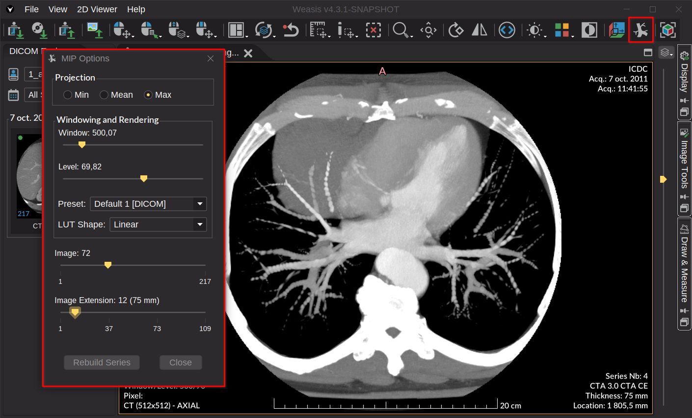
MIP options
The MIP options panel can be opened from either of two places:
The
button in the Basic 3D toolbar — applies to the currently selected view.
The
indicator in the top-right corner of any view that already has MIP active.
Note
Annotations and measurements can be added on a MIP-projected image, but they are not persistent when scrolling: each annotation is tied to the exact slice position on which it was drawn, and disappears as soon as you navigate away. To keep annotations attached to a specific MIP configuration, build a new series from those options.
Projection
The projection type controls how each pixel of the output is computed across the slab:
None — no projection; display the original image.
Min — Minimum Intensity Projection.
Mean — Mean Intensity Projection.
Max — Maximum Intensity Projection.
Switching from None to any of the projection types initializes the slab thickness to 2 slices (2 slices before and 2 slices after the current one).
MIP thickness
Defines the extent of the slab used for the projection — expressed as a number of slices before and after the current one (e.g. a value of 3 means 3 slices on each side of the current slice, 7 slices total in the slab).
The dropdown shows suggested values, with the corresponding physical thickness in millimeters shown in parentheses when the series is spatially calibrated (e.g. 5 (3.5 mm)). The last entry, Custom thickness, lets you type any value manually.
Build a new series
Builds a new MIP series from the current options — every slice of the source series is reprojected with the chosen projection type and slab thickness, and the result is stored as a standalone series. The new series is added to the DICOM Explorer and can be exported like any other series. Annotations drawn on the new series are persistent since they are no longer tied to a live slab calculation.
Image Fusion
Image Fusion
Image fusion overlays a functional series — PET (PT) or SPECT (NM) — on top of an anatomical CT or MR base, so metabolic uptake can be read against the underlying anatomy. The overlay is a registration-free geometric fusion: Weasis aligns the two series from their DICOM spatial metadata alone, with no manual or algorithmic registration step. Available since Version4.7.1.
Note
Fusion is a pure spatial overlay driven by each image’s position in the patient coordinate system. It does not deform or re-register the images, so it is only offered when the two series are genuinely co-located (see Requirements below).
Requirements
A series can be fused onto the displayed base only when all of the following hold:
Condition
Detail
Modality pairing
A functional overlay (PT, NM) on an anatomical base (CT, MR).
Same study
Both series share the same StudyInstanceUID.
Volume geometry
Both are cross-sectional volumes (≥ 2 slices with Image Position / Orientation Patient and Pixel Spacing).
Same coordinate system
Either the FrameOfReferenceUID matches, or — as is common for separately reconstructed PET/CT — the two volumes overlap in patient space.
When no compatible overlay is found in the study, the fusion controls stay disabled.
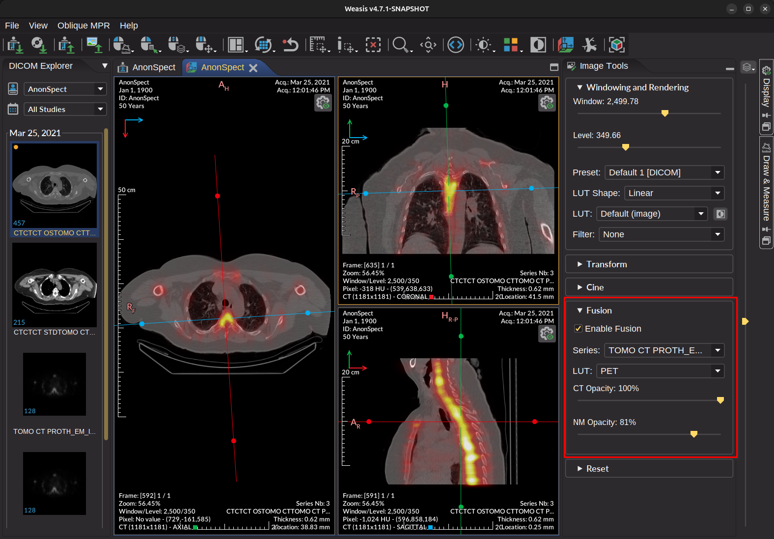
Enable fusion
The fusion controls live in the Fusion section of the Image tool
panel. The section is collapsed by default — click its header to expand it.
Enable Fusion — turns the overlay on or off. The other controls become active only while fusion is enabled.
Series — the functional series to overlay. The list contains every compatible overlay found in the current study (see Requirements).
LUT — the color lookup table applied to the overlay. PET (a hot-metal palette tuned for functional data) is selected by default. The overlay is colorized through the functional series’ own window/level, so it shows exactly the colors the overlay would have if displayed directly with that LUT.
Opacity — two sliders set a flat blend (cross-fade) at composite time: result = baseOpacity·base + overlayOpacity·overlay. Each is labelled with the modality of the layer it controls (e.g. CT for the base, PT for the overlay). Defaults are 100 % base and 75 % overlay. Setting base 0 % and overlay 100 % shows the pure colorized overlay, identical to the functional series viewed on its own with the same LUT.
The overlay follows the base view as you scroll, zoom, window, or reslice it. Because the fusion is resampled from the functional volume, it stays correct on oblique, coronal and sagittal planes, not only the native acquisition plane.
Note
The Reset action turns fusion off and returns to the plain base image, like any other display setting it restores.
SUV statistics on a region of interest
When the overlay is a PET series carrying the required metadata, a closed measurement drawn on the fused base image also reports the overlay’s SUV values inside the region — Min, Max and Mean, in SUVbw, g/ml. These rows are sampled from the original PET voxels (no resampling loss on the maximum) and are tagged with the overlay’s modality — for example Max (PT) — so they read alongside the base-image statistics.
Tip
SUV is computed with the body-weight method (SUVbw), following the vendor-neutral QIBA definition. The same values can be read directly on the PET series itself — see SUV measurements.
Fusion in the MPR viewer
Opening the MPR viewer from a fused 2D view carries the fusion over: the three MPR planes start with the same overlay series, LUT and opacities you set in the 2D view. Each plane keeps its own fusion settings, so you can fine-tune — or disable — the overlay independently per plane afterwards, without affecting the 2D view or the other planes.
Note
Inheritance only applies when the overlay is still compatible with the reconstructed MPR base. If you open MPR from a non-fused view, the planes start with fusion off, and you can enable it from the same Fusion section as in the 2D viewer.
The 3D viewer reconstructs a CT, MR, PET, or other volumetric series into an interactive volume rendering that can be rotated, sliced, recolored, and lit in real time. Typical uses include reviewing CT angiography, inspecting bone or vascular anatomy, surgical-planning views, and quickly conveying findings to colleagues or patients. Available since Version4.1.0, with major rendering and synchronization improvements in Version4.7.0.
Internally, the volume is rendered on the graphics card using a ray-casting algorithm implemented in GLSL shaders, so a modern GPU is required (see Requirements) but no extra installation step is necessary.
Requirements
The graphics-card capabilities used by Weasis are reported under OpenGL Support in File > Preferences > Viewer > 3D Viewer:
Driver version — requires OpenGL 3.3+ since Version4.7.0. Two rendering backends are used depending on the available OpenGL version:
OpenGL 4.3+ — uses a Compute Shader for optimal performance.
OpenGL 3.3 – 4.2 — uses an FBO-based Fragment Shader fallback (fully functional, but may be less performant than the Compute Shader path). macOS is capped at OpenGL 4.1 and therefore always uses this path.
Max 3D texture dimension length — the upper limit, in voxels, of any X / Y / Z dimension of the volume.
Any other entry shown in red indicates a non-optimal configuration. The viewer often still works — see how to limit the size of 3D textures if performance becomes an issue.
Note
If Weasis reports a graphics card that is not the one you expected, the choice is made by the graphics driver and the operating system, not by Weasis. OpenGL itself has no API to select a specific card; consult your OS’s GPU-selection settings for the application.
Open the 3D viewer
Open the viewer by clicking
in the toolbar of a series view, by double-clicking the series thumbnail, or by right-clicking the thumbnail in the DICOM Explorer and choosing the 3D viewer.
Tip
If the series is a multi-phase 4D acquisition (e.g. a cardiac CT with several temporal phases), Weasis automatically splits it into individual phase sub-series when 2–7 phases are detected. For series with 8 or more phases, a confirmation dialog is shown first. Open any resulting phase sub-series to render it in the 3D viewer. See 4D Series Sub-Series Splitting for details.
Try it on a volume dataset (Medical Demos from data.kitware.com)
Launch
Reload volume — fully reloads the volume from the source series.
Orthographic / Perspective projection — toggles between orthographic projection (parallel lines preserved, no foreshortening — useful for measurements) and perspective projection (depth cues, more natural-looking view). Perspective is the default.
MPR Crosshair Cut — opens the cut mode to interactively clip the rendered volume along the anatomical planes defined by the MPR crosshair.
Other toolbar buttons (LUT, reset, layout, synchronize…) are documented in the sections below.
MPR Crosshair Cut Mode
Since Version4.7.0 the 3D viewer can display an MPR crosshair overlay synchronized with the MPR viewer, allowing you to clip the rendered volume along the anatomical planes defined by the crosshair position and orientation. The crosshair position and rotation stay synchronized in real time between the 2D MPR planes and the 3D rendering.
In the MPR toolbar, click
— this splits the current tab into a side-by-side layout with the MPR views on one side and the 3D volume rendering on the other.
In the 3D view, activate a cut mode using the toolbar button
or by right-clicking and selecting MPR Crosshair Cut.
Alternative workflow
Open the 3D viewer first, then activate a cut mode from the toolbar
or the right-click menu. The MPR viewer opens automatically for the same series, but in a separate tab. To obtain the side-by-side layout, drag the MPR tab and dock it next to the 3D view using the docking handles.
Cut modes
No cut — no clipping; the full volume is rendered.
18 directional modes — clip the volume in halves, quarters, or eighths relative to the MPR crosshair position, along each anatomical axis (Left / Right, Anterior / Posterior, Superior / Inferior).
The crosshair overlay uses the same LPS axis color coding as the MPR viewer.
3D View Synchronization
Since Version4.7.0 the 3D viewer can host multiple side-by-side views of the same volume and keep them coordinated. Because every 3D view in the container shows the same volume, the auto-sync button
is always visible. A single synchronization profile bundles a per-action toggle list with camera-level actions enabled by default and photometric / rendering actions left opt-in.
Toolbar “Synchronize” checkbox
The
Synchronize checkbox in the toolbar drives the global on/off state for the 3D container. It defaults to ON. Toggling it propagates the new state to every per-view auto-sync button on the next refresh.
Per-view auto-sync button
When the layout has two or more views, a small auto-sync button appears in the bottom-right corner of each view. Its tint reflects the per-view state — red when sync is OFF for the view, green when ON. Clicking the button opens a popup with:
Synchronize this view — master on/off toggle for auto-sync on this view (also mirrored into the toolbar Synchronize checkbox so the toolbar state always reflects the active view).
Per-action toggles — independent checkboxes that decide which actions this view propagates to (and receives from) the other 3D views. The popup stays open while you flip several options.
Apply to all views — copies this view’s effective per-action map to every other 3D view in the container. Unlike the 2D variant of this entry, no FoR filtering is applied because all 3D views share the same volume.
Right-click “Synchronize” submenu
The view’s right-click context menu also exposes a Synchronize submenu with the same per-action toggles and the same Apply to all views entry, useful when you want to adjust the sync map without first enabling/disabling the master toggle.
Per-action defaults
Group
Action
Default
Camera
Pan
ON
Camera
Zoom
ON
Camera
Rotation (slider rotation + axis selection)
ON
Photometric
Window / Level
OFF
Photometric
Preset
OFF
Photometric
LUT Shape
OFF
Photometric
Invert LUT
OFF
Photometric
LUT
OFF
Rendering
Rendering Type
OFF
Rendering
Volume Opacity
OFF
Rendering
Volume Shading
OFF
Rendering
Orthographic projection
OFF
Rendering
MPR Crosshair Cut
OFF
Camera-level actions are on by default because keeping multiple 3D views framed identically is the common workflow when comparing rendering types or LUT presets side by side. Photometric and rendering actions are opt-in because the typical reason to open a second 3D view is to diverge on those settings (e.g. one view in Composite with a soft-tissue LUT, the other in MIP).
Note
The view you are actively interacting with always applies its own changes locally, even when the corresponding action is unchecked in its sync map. Only other views gate on the per-action toggle. This keeps sliders and mouse drags responsive while letting you decide which actions propagate to the rest of the container.
3D Rendering Tools
This tab groups every control that affects how the volume is rendered. To return to the original settings, click the toolbar button
or pick Reset from the context menu.
Windowing and Rendering B
Some of the options below are also accessible from the toolbar and the right-click menu.
Window — width of the voxel-value range mapped to the displayed value range.
Level — center of the range defined by Window.
LUT Shape — transfer function applied between input and display values: linear, sigmoid, or logarithmic. Default is linear.
LUT — a 3D Lookup Table that maps grayscale voxel values to color, opacity, and lighting for visualization. Picking a LUT from the toolbar or the right-click menu is usually easier: LUTs there are ordered by modality and shown with a preview.
Invert LUT — flips the LUT direction.
Volume Rendering C
Controls for the rendering algorithm, quality, transparency, lighting, and shading.
Type — defines the rendering algorithm applied to the volume:
Composite — classic volume rendering. Each voxel contributes color and opacity along the ray, blended front-to-back to produce the final image.
MIP Max — Maximum Intensity Projection. Keeps the highest-intensity voxel encountered along each ray. Useful for highlighting bright structures such as contrast-enhanced vessels or bones.
MinIP — Minimum Intensity Projection. Keeps the lowest-intensity voxel along each ray. Useful for visualizing air-filled structures such as airways.
MIP Mean — Mean Intensity Projection. Averages intensities along each ray, producing a smoother representation of the volume.
Iso Surface — renders a 3D surface at a given intensity threshold, representing structures of a uniform density (e.g. bone segmentation).
Z-axis sampling — distance between successive samples along each ray. Smaller values capture more detail at the cost of compute time; the default is derived from the volume size.
Opacity — global opacity factor for the voxels. Can be pushed above 100 % to compensate for the lower-than-100 % values defined by some Volume LUTs.
Shading — enables shading on the rendered surface. The default is taken from the Volume LUT; the additional options let you override the inherited lighting settings.
Transform D
Zoom the volume and rotate it around the three patient axes:
Zoom slider — scales the rendering.
Rotation sliders — rotate around the Left / Right, Anterior / Posterior, and Superior / Inferior axes (LPS coordinate system).
Preferences
From the menu File > Preferences > Viewer > 3D Viewer.
OpenGL Support
Information about the graphics card and OpenGL capabilities, see Requirements.
3D Viewer
Default layout — preferred layout used when opening the 3D viewer. Available layouts: 1×1 (single view, default), 1×2, 2×1, 1×3, 2×2.
Max 3D texture size — maximum volume dimensions, both in X / Y (image width and height) and in Z (number of images in the stack composing the volume).
Note
The maximum 3D texture defaults come from the graphics card. Lowering them (e.g. to 512) can produce a more fluid rendering on hardware that struggles with the full-size texture.
Volume Rendering
Dynamic quality — reduces the rendering quality along the Z axis while you rotate or modify the view, for a smoother interaction. At the maximum slider position there is no quality reduction.
Default orientation — preferred starting orientation. Default: anterior view rotated 15° to the right and 15° downward.
Background color — background color of the rendered scene.
Light color — color of the light used to illuminate the rendering.
Video tutorials
Display an MR angiography series as a volume rendering, then switch to a MIP projection or pick a 3D LUT and adjust the window / level values:
DICOM ECG Viewer
Displaying electrocardiography data
The ECG viewer displays and analyzes electrocardiogram waveforms stored as DICOM Waveform objects — resting and stress 12-lead ECGs, ambulatory recordings, and rhythm strips. It also provides simple on-screen calipers for measuring intervals and amplitudes, with support for the common lead layouts (12-lead, 3-lead, rhythm strip).
Waveform Annotations — measurements, classifications, regions of interest, or events that may affect interpretation (for example, the timestamp at which the subject coughed or moved).
DICOM SR Viewer
Displaying DICOM Structured Report
A DICOM Structured Report (SR) carries structured findings — measurements, observations, classifications, and references back to the images they were derived from — as a hierarchical tree of content items rather than free-form text. SRs are produced by radiology reporting systems, ultrasound machines, CAD applications, and increasingly by AI inference frameworks that need to expose machine-readable results.
Weasis renders the SR tree on the right and the image referenced by the currently selected item on the left, so you can read a finding and inspect the underlying image at the same time.
Show DICOM metadata — open the full DICOM attributes of the SR object.
Display SR Header B
The SR header is displayed as a three-column table summarizing the patient identification, the study context, and the report status (e.g. Partial, Complete, Verified, Cancelled).
DICOM SR Tree C
The content of the SR is displayed as a hierarchical tree. Each node is a content item with its own number, a concept name (what the item describes — e.g. Finding Site, Length, CAD Output) and a value (text, code, numeric measurement, date/time, image reference, or composite reference). The hierarchy and the inter-item links mirror the relationships defined in the SR object — typically following one of the standard DICOM templates (TIDs) used in radiology, ultrasound, or AI reporting.
Some items also carry a link to a referenced image or region. Clicking such a link opens the corresponding image in the 2D viewer and, when the SR contains coordinate data, draws the referenced geometry on top of it (for example, clicking the POLYLINE node in the screenshot above opens the source image and displays the polyline measurement at its recorded position).
Weasis renders the standard SR graphic types — POINT, MULTIPOINT, POLYLINE, CIRCLE, ELLIPSE — and, since v4.7.0, a subset of the SR compound graphic types — MULTILINE, RULER, ARROW, RECTANGLE — for richer overlays carried by the SR Compound Graphic module.
DICOM Audio Player
Playing DICOM AU data
The DICOM Audio SOP Class (commonly referred to as DICOM AU) stores waveform audio inside a DICOM object. It is most often used for voice annotations dictated by the technologist or radiologist, Doppler ultrasound audio, phonocardiography, and other acoustic signals captured alongside an imaging study.
Weasis opens these objects in a dedicated player launched by double-clicking the audio thumbnail in the DICOM Explorer.
Show DICOM metadata — opens the DICOM attributes of the audio object.
Play B
The Play button toggles between playback and pause. The slider lets you scrub through the recording; the current position is displayed in seconds.
Volume C
Adjusts playback volume independently of the system mixer.
Export Audio File D
Saves the embedded waveform to disk as either:
AU — the format used by the DICOM payload itself, preserved as-is.
WAVE (.wav) — re-encoded for broad compatibility with consumer audio players and editors.
Draw & Measure
How to draw and measure on images
The Draw & Measure panel lets you annotate and measure on DICOM and standard images — distances, angles, areas, regions of interest, free-hand shapes, and text labels. Measurement values are computed from the image’s spatial calibration when available, and from pixel statistics when the shape is closed.
Where the results are persisted depends on the image type:
For DICOM images — saved into a DICOM Presentation State (GSPS) object that travels with the study.
For standard images — saved into an XML file in the same directory as the image (when the image is exported in a non-DICOM format). The XML file is loaded automatically the next time the image is opened in the 2D viewer.
Draw & Measure Panel
Click
on the vertical button
to dock the panel on the right side of the viewer. The panel is divided into four parts:
Click a measurement tool and then draw on the image. Picking a tool here also becomes the active action on the left mouse button.
The first button is the selection tool — used to select, resize, and move existing graphic objects.
Once one or more graphics are selected, you can change their properties (color, line width…) or copy/paste them through the right-click menu. The selection can be removed with the Delete key or
. See the full list of graphic shortcuts.
Note
A segment can be drawn in two equivalent ways:
Click + Drag — click, drag to draw, release.
Click > Release > Drag — click to set the start point, release, drag to draw, click again to set the end point.
To keep the same tool active for several draws in a row, uncheck Draw only once (see Graphic Options).
Tip
For a polyline or polygon, double-click to finish editing. Right-clicking a vertex offers add / delete actions on that specific point.
Rectangles and ellipses can be drawn at any angle. The external control points rotate and resize the shape; the single control point on the opposite side resizes only.
Drawings B
The drawing buttons add text and graphic annotations. These objects are purely decorative — they do not display measurement values and do not appear in the Selected Measurement table.
Graphic Options C
Line color — default color for new graphics (default: yellow). The transparency / alpha slider in the color picker controls opacity.
Line width — default line width.
Draw only once — when checked, the tool reverts to the selection mode after each draw. Uncheck to keep the same tool active for successive draws.
Pixel statistics — compute and display statistics of the pixel values inside the shape. Only meaningful for closed shapes (rectangle, ellipse, polygon).
Unit — unit of the image’s spatial calibration. When the image has no calibration, the unit falls back to pixels. See How to change the spatial calibration.
More options — opens the Draw & Measure preferences for the deeper display options.
Tip
All graphics can be shown or hidden at once from the Display panel by checking or unchecking the Drawings option.
Selected Measurement D
The graphic E currently selected on the image is summarized in this table. The reported properties depend on the measurement type, with units shown in square brackets when present (see the calibration type at M).
Note
For polygons, length, width, and orientation are computed with the OMBB (Oriented Minimum Bounding Box) method — a tighter bounding box than the axis-aligned one, giving a more accurate approximation of the polygon’s real dimensions.
When Pixel statistics is checked, the table also reports descriptors computed from the pixels enclosed by the (closed) shape:
Pixels — number of pixels inside the shape.
Min — minimum modality value.
Max — maximum modality value.
Median — median modality value.
Mean — mean modality value.
StDev — standard deviation; a measure of how dispersed the values are.
Skewness — asymmetry of the value distribution.
Kurtosis — “tailedness” of the value distribution.
Note
SUV (Standardized Uptake Value) measurements are added to the table on PET images when the required metadata is present (patient weight, decay correction, radiopharmaceutical dose, acquisition time, …). Min / Max / Mean SUV are computed with the body-weight method (SUVbw), following the vendor-neutral QIBA definition.
Tip
The table can be exported by copy / paste. The copied values use the full numerical precision, not the rounded values shown on screen.
Preferences
From the main menu File > Preferences > Draw & Measure.
Drawings
Default graphic properties applied when drawing new objects — since Version4.3.0.
Line color — default color (default: yellow). The transparency / alpha slider in the color picker controls opacity.
Line width — default line width.
Fill shape — when checked, the interior of the shape is filled with the line color.
Fill opacity — opacity of the interior, relative to the line color’s opacity. Default: 100 %. Example: line opacity 80 % × fill opacity 20 % → perceived interior opacity 16 %.
Labels on image
Display options for the labels attached to measurement graphics.
Font type — default font size for the on-image labels (default: Small semibold). The size is not absolute — it adjusts automatically with the interface scale factor.
Geometric measurement — which geometric measurements are displayed on the image for each graphic type.
Pixel statistics — which pixel statistics are displayed on the image for closed shapes (rectangle, ellipse, polygon).
DICOM RT Tools
Displaying radiotherapy information
Radiotherapy treatment data is distributed across three companion DICOM objects:
RTSTRUCT — contoured structures (target volumes, organs at risk, body outline) referenced to a planning CT.
RTPLAN — prescribed dose, fractionation, beam geometry, and machine setup.
RTDOSE — the computed dose distribution as a 3D pixel grid, with optional pre-computed DVH histograms.
When a CT series is loaded together with its associated RTSTRUCT, RTPLAN, and RTDOSE files, Weasis automatically links them and the RT Tool appears in the right panel.
How to display structures
Click Load RT to load the linked DICOM STRUCT, PLAN, and DOSE objects. The button becomes inactive once loading completes.
InfoOptional Select a structure set if more than one is available.
InfoOptional Select a plan if more than one is available.
The region tree exposes a context menu with the following actions:
Select / unselect all child nodes (parent nodes only) — toggle visibility for every sub-region in a group at once.
Fill opacity — controls the transparency of the region’s interior relative to its border.
Default value: 20%
Perceived opacity = Line opacity × Fill opacity
Example: 80 % line + 20 % fill → 16 % perceived interior opacity.
Export to clipboard as CSV — copies region data (volume measurements, dose calculations) for analysis in spreadsheets or external tools.
Pixel statistics from the selected view (leaf nodes only) — computes statistical descriptors of pixel values inside the region. For the parameter definitions, see Pixel Statistics.
How to display isodoses
Switch to the Isodoses tab.
Check the Isodoses root node — it is unchecked by default.
InfoOptional Adjust the graphic opacity (default: 50 %).
Tip
The Structures and Isodoses root nodes act as master switches — toggle them to show or hide all overlays at once, while child nodes keep individual control over specific items.
Note
Since Version4.7.0 the isodose overlay is rendered directly from the RTDOSE pixel grid (resampled to the CT image grid using nearest-neighbor interpolation) instead of vector contours. This provides a more faithful representation of the dose distribution stored in the DICOM file, especially around steep dose gradients.
How to display the DVH chart
The Dose-Volume Histogram (DVH) summarizes, for each selected structure, the fraction of its volume that receives at least a given dose level — the standard way to compare plans and check organ-at-risk constraints.
Select one or several structures (the Structures root node must also be selected).
Click Display DVH chart.
Right-click on the chart to print or save as PNG, or as a vector file (SVG, EPS).
Warning
Since Version4.7.0, when one or more selected structures have no DVH stored in the RTDOSE, a confirmation dialog lists the affected structures and offers to compute the missing histograms on the fly.
The calculation algorithm (derived from dicompyler) is experimental and not clinically validated: results must not be used for medical decisions. The feature can be disabled by setting the system preferenceweasis.rt.dvh.recalculate.enable to false; when disabled, only DVHs already stored in the RTDOSE are displayed.
DICOM Attributes
How to display DICOM attributes
Every DICOM object carries a set of attributes (also called tags or metadata) that describe the patient, the study, the acquisition device, the imaging parameters, and so on. Weasis can display these attributes in two ways — a dynamic in-layout view that follows the current image, or a detached window snapshot of a single instance.
Opening the DICOM attributes
Open the DICOM attributes either by:
selecting the DICOM Information layout from the layouts dropdown A, or
clicking the DICOM Information button
in the toolbar to open a detached window B.
Note
The two display modes behave differently when you scroll:
In-layout view (A) — the attributes are updated dynamically and reflect the currently displayed image (useful while scrolling through a series).
Detached window (B) — the attributes are a snapshot of the instance that was active when the window was opened. They do not update when you scroll.
When Weasis opens certain DICOM payloads with an external application (e.g. encapsulated PDF or video), the attributes can still be inspected from the thumbnail right-click menu.
How to find a specific DICOM attribute or value
The DICOM Information window has two tabs:
Limited DICOM attributes — the main attributes grouped by category (a curated subset for everyday use).
All DICOM attributes — every attribute present in the file. Each data element is shown in four columns: Tag ID, VR, Tag Name, Value.
Note
When a data element holds multiple values, they are separated by a single backslash \.
Data elements whose Value Representation (VR) is one of OB, OD, OL, OF, OW, or UN — binary VRs used for pixel data, lookup tables, and other large byte streams — display binary data in place of the actual bytes.
The example above searches for the word date. The procedure is:
Switch to the All DICOM attributes tab so every attribute is searchable.
Type the search term in the search field.
Use the navigation arrows to jump between highlighted matches. The rightmost button filters the list to only the matching rows (instead of just highlighting them inside the full list).
Using in the toolbar applies a persistent filter on the attribute list — useful when you want to keep the focus on a specific set of attributes while scrolling through a stack of images (in-layout view A) only).
Note
Some attributes are nested inside a sequence element (marker (5) in the screenshot). The arrow on the left of a row shows the nesting depth — sequences can themselves contain sequences.
Tip
When a value is too long to fit:
Resize the column from its header — the new width is kept until the displayed image changes.
Hover the cell to read the full value as a tooltip (since Version4.3.0).
Tip
The selected DICOM attributes can be copied to the clipboard with the standard copy shortcut of your operating system. Paste into a spreadsheet, a text editor, or a bug report.
Lookup Tables (LUT)
How to handle Color and DICOM LUTs
A Lookup Table (LUT) maps each input pixel value to an output value used somewhere along the rendering pipeline — turning raw acquisition numbers into the contrast, the color, and the brightness you actually see on screen. The DICOM rendering pipeline chains four kinds of LUT, each applied at a different stage:
Modality LUT — converts raw pixel values into physical modality values (e.g. Hounsfield units for CT).
Values of Interest (VOI) LUT — maps the modality values into a visible intensity range, enhancing specific anatomical structures or pathological conditions (this is what the Window / Level controls).
Presentation LUT — converts the intensity values into P-Values: device-independent values calibrated to human perception (used to render consistently across monitors).
Palette Color LUT — replaces grayscale intensity values with colors, producing a pseudo-color rendering.
Note
The Modality LUT and the Palette Color LUT are applied automatically when present in the DICOM file — there are no controls in the user interface to override them.
Windowing and Rendering
Windowing and Rendering is a panel in Image Tools of the 2D viewer, exposing the user-controllable parts of the LUT pipeline. The same controls are also accessible from the Lookup Table toolbar, the main menu, and the right-click menu.
Window — width of the input range mapped to the displayed values. Change it via the slider, or by selecting Window / Level in the mouse actions.
Level — center of the range defined by Window. Same input options as above.
Preset — picks a predefined Window / Level pair. The dropdown is ordered as:
An empty entry, shown while Window and Level are being adjusted manually (slider or mouse drag).
Window / Level pairs or VOI LUT data carried by the DICOM file (suffixed with [DICOM]). The default selection is the first [DICOM] entry when present, otherwise Auto Level [Image].
Auto Level [Image] (always shown) — Window and Level computed from the full pixel-value range of the current image.
Modality-specific presets (e.g. Lung, Bone, Soft Tissue for CT).
LUT Shape — the transfer function used between input and display: linear (default), sigmoid, or logarithmic.
LUT — pseudo-color LUT applied on top of the grayscale image. Default (image) keeps the original image color model. Picking a LUT from the toolbar or the menus is usually easier because each entry is shown with a preview.
Invert LUT — flips the LUT direction (dark↔bright, or reversed color mapping).
Filter — 2D image filter applied before the LUT, useful for enhancing image quality or highlighting specific structures. Default: None.
Tip
To overlay the active LUT bar on the image, enable it from the Display panel on the right. The values labeled on the bar correspond to the Modality LUT values (e.g. Hounsfield units for CT) when one is defined, or to raw pixel values otherwise.
To inspect how the current Window / Level reshapes the pixel distribution, switch to the Histogram layout.
Build DICOM KO and PR
How to build and export DICOM KO and PR
Weasis can author two standard DICOM annotation objects directly from the viewer:
Key Object Selection (KO) — a list of “key images” inside a series. Use it to flag the slices that matter for a finding so a reader can scroll only through those.
Presentation State (PR / GSPS) — drawings, measurements, and other graphic overlays that reference the source images. Use it to share findings across systems without baking annotations into the pixels.
Both objects can be saved as proper DICOM files and sent to a PACS through the standard DICOM Export workflow, so they travel with the study and can be re-applied by any DICOM-compatible viewer.
Key Object Selection (KO)
To make the KO controls visible, enable the Key Object Selection toolbar from View > Toolbars > Key Object Selection Toolbar in the main menu.
When a DICOM KO is loaded with the series, it appears in the explorer menu (1) and can also be picked from the icon on the right side of the view (6). KO objects created in Weasis behave the same way.
Actions available in the KO toolbar:
Apply a KO (2)
— select which KO drives the current view.
Mark / unmark a key image (3) — click the star icon, or press K (default — customizable since v4.7.0 in Keyboard Shortcuts) to add the current image to the active KO, or create a new one if none exists yet.
Filter to key images only (4) — when active, scrolling skips every image that is not part of the selected KO, so you see only the flagged slices.
Create / delete a KO (5) — start a new KO (optionally seeded from an existing one) or delete a KO. Only KOs created by Weasis can be deleted.
Presentation State (PR or GSPS)
Apply a PR loaded from a DICOM file (1)
— since Version2.6.0, PRs are not applied automatically; click the dedicated icon (2) above the image to apply one. To have the most recent PR applied by default, enable Apply by default the most recent Presentation State under File > Preferences (Alt + P) (also configurable through the default preferences).
Create a new PR — any drawing or measurement (see Draw & Measure) can be exported into a DICOM Presentation State. Image-rendering parameters (zoom, calibration, window/level, LUT…) are not yet included in the exported PR.
Exporting Key Object Selection or Presentation State
Newly created KO and PR objects are exported through the standard DICOM Export dialog — open it from the toolbar icon or from File > Export > DICOM.
Pick the export destination — Local Device, DICOM Send, or CD/DVD Image (see DICOM Export for the per-destination options).
Choose the export options. Series created inside Weasis (including new KO and PR objects) are flagged NEW in the selection tree.
Select the patient(s), study, series, or individual instances to export.
Click Export to write or transfer the files, then close the window.
DICOM SEG
Displaying DICOM Segmentation
DICOM Segmentation (SEG) stores pixel-based labels — anatomical structures, lesions, organs at risk — as a separate object that references a source image series. It is the standard delivery format for AI segmentation frameworks, but also for manual or semi-automatic contouring tools.
Weasis displays SEG regions as a colored overlay on the source images, with independent visibility and opacity control per region. Available since Version4.3.0; significantly extended in Version4.7.0 with:
Overlays in MPR and 3D Volume Renderer views, in addition to the standard 2D viewer.
Simultaneous display of all SEG files linked to the current series, each toggleable independently.
Support for the FRACTIONAL (probability / occupancy maps) and LABELMAP (multi-segment files used by tools like highdicom) segmentation types produced by modern AI frameworks.
The same smooth fractional overlay reused for RT Dose isodose rendering — see the RT tutorial.
How to display DICOM SEG in the 2D viewer
To display the SEG regions as an overlay on the image, follow these steps (see the image below):
Open a DICOM series that has a linked SEG object. The link is indicated by the segmentation icon
in the lower-right corner of the thumbnail.
Once the image is displayed, click
on the vertical
button to open the Segmentation panel on the right side of the viewer.
Every SEG file linked to the current series appears as a top-level node in the tree. Expand a SEG node to reveal its regions and tick the ones you want to display. Regions that share a common name prefix are grouped under a parent node — the parent must be checked for any of its children to be visible.
InfoOptional Adjust the global graphic opacity (border and interior fill) with the slider.
InfoOptional Use tooltips to see the region description, voxel count and estimated volume for each region. For FRACTIONAL regions a color-gradient bar is also displayed to help interpret the probability ramp.
Select / unselect all child nodes (parent only) — toggle visibility for every child region at once.
Fill opacity — transparency of a region’s interior relative to its border.
Default: 20 %
Perceived opacity = Line opacity × Fill opacity
Example: 80 % line + 20 % fill → 16 % perceived interior opacity.
Show in the image view (leaf only) — jumps to the slice where the region has its largest cross-section.
Pixel statistics from the selected view (leaf only) — computes statistical descriptors of pixel values inside the region. For the parameter definitions, see Pixel Statistics.
Note
Loading a DICOM SEG. The first time a SEG is shown — in the 2D viewer, MPR or 3D — Weasis decodes it in the background. Scrolling and other interactions remain responsive while decoding runs; the regions appear as soon as the SEG is ready.
A cancelable progress entry is shown at the bottom of the DICOM Explorer, so a large or slow SEG can be canceled without blocking the rest of your work.
Once decoded, the SEG is shared between the 2D, MPR and 3D views — loaded only once even with several views open. Weasis may release it automatically when memory gets tight and reload it on demand the next time it is needed.
Supported segmentation types
Weasis supports all three DICOM SEG segmentation types:
Type
What it represents
How Weasis displays it
BINARY
Each pixel is either inside or outside the segment.
Colored contour drawn on the image.
FRACTIONAL — PROBABILITY
Each pixel carries a value between 0 and 1 expressing how confident the AI is that the pixel belongs to the segment.
Smooth colored overlay: more transparent where confidence is low, more opaque where it is high. The opacity slider scales the whole gradient.
FRACTIONAL — OCCUPANCY
Each pixel carries a value between 0 and 1 expressing how much of the pixel is actually covered by the segment (partial-volume fraction).
Same smooth overlay as PROBABILITY — only the meaning of the value differs.
LABELMAP
Several segments are packed into a single image, with the pixel value identifying which segment it belongs to.
Each segment is extracted automatically and drawn with its own color.
Note
Some AI frameworks export FRACTIONAL segmentations without an explicit reference back to the source series. Weasis matches them to the correct images automatically (via the DICOM frame of reference).
Segmentation overlay in MPR
When a DICOM SEG is linked to the current series, the overlay is automatically available in the Multi-Planar Reconstruction (MPR) view. The same Segmentation panel controls visibility and opacity for all three planes (axial, coronal, sagittal — plus any oblique cut) at once.
For MPR, Weasis additionally has to reslice the SEG along the new planes. This extra step runs in the background; the overlay appears on every plane as soon as it completes.
Tip
The MPR overlay works even when the SEG has a different orientation, spacing or scanning direction than the source images — for example an AI model that segments at a coarser resolution. Weasis reprojects the mask into the image coordinate system, so contours stay aligned on every plane.
Segmentation overlay in the 3D Volume Renderer
The 3D Volume Renderer offers three segmentation modes, selectable from the Segmentation panel:
Mode
What it shows
No segmentation
Volume rendering only — no overlay.
Segmentation only
Only the labeled regions are rendered; the anatomy is hidden. Useful to review the AI output on its own.
Segmentation overlay
Regions are drawn on top of the volume rendering, with the anatomy remaining visible beneath.
A few things to keep in mind when working with the 3D overlay:
Toggling a segment is instant. Visibility, color and opacity changes update the 3D view immediately, even on very large volumes — Weasis only refreshes the color table, not the segmentation itself.
Overlapping segments are handled cleanly. When two segments share the same area, their colors are blended automatically; you do not have to pick which one wins.
2D, MPR and 3D stay in sync. Showing or hiding a segment in the panel updates all three views simultaneously.
AI DICOM Objects
DICOM objects generated by artificial intelligence
AI inference rarely defines its own file formats — instead, results are packaged as standard DICOM objects so any compliant PACS or viewer can ingest them. The same SOP Classes used for human-authored content (segmentations, structured reports, presentation states…) are reused to carry model outputs.
This page maps the AI-produced object types you are most likely to encounter to how Weasis displays them.
These objects carry their own pixel data and are viewed as standalone images.
DICOM Secondary Capture (SC)
Pre-rendered images where the AI has burned its output directly into the pixels — typically annotations, heatmaps, or side-by-side comparisons. Convenient for legacy viewers, but the overlay cannot be toggled off or recomputed.
Info
Secondary Capture displays like any other image, see DICOM 2D Viewer.
DICOM Enhanced Objects
Reconstructed or post-processed images — for example denoised CTs, super-resolved MRs, or motion-corrected series. The output replaces or complements the original acquisition rather than annotating it.
Info
Enhanced images display like any other image. Overlays, shutters, and pixel padding stored in the object are honored by the rendering pipeline — see 2D Viewer Display.
DICOM Parametric Map (PMAP)
Single- or multi-frame images whose pixel values represent a derived quantity rather than an acquisition signal — common carriers for AI probability maps, class-activation heatmaps, perfusion (rCBF, rCBV, MTT), diffusion (ADC), and PET-derived metrics.
Info
Weasis renders Parametric Maps as standard images, including the float and double pixel representations that AI pipelines typically emit. Window/level and LUT controls apply normally — pick a suitable LUT to interpret the value range.
Image overlays
These objects do not contain a viewable image of their own; they reference a source series and are drawn on top of it.
DICOM Segmentation (SEG)
Pixel-based labels produced by segmentation models — anatomical structures, lesions, organs at risk, etc. Each segment is stored as a binary or fractional mask and is independently toggleable in the viewer.
Info
See DICOM SEG for displaying DICOM SEG objects in Weasis, including in MPR and the 3D Volume Renderer.
DICOM RTSTRUCT
Originally designed to describe contours for radiotherapy planning, RTSTRUCT is also used by AI tools that output vector geometry instead of pixel masks. Lighter to store than SEG, but inherently 2D per slice.
Info
See DICOM RT for displaying DICOM RTSTRUCT objects in Weasis.
TotalSegmentator is a good example: starting from version 2, its automatic segmentation of 100+ anatomical structures on CT can be exported as DICOM RTSTRUCT — and, in recent releases, as DICOM SEG as well — both of which load directly in Weasis without any extra configuration.
DICOM Presentation States (GSPS)
Grayscale Softcopy Presentation States store the display intent for an image — window/level, zoom, rotation — together with vector annotations and measurements. AI tools use them to ship findings as toggleable overlays on the original images rather than baking them into pixels.
Info
See DICOM PR for displaying DICOM Presentation States in Weasis.
Reports & documents
These objects carry structured or document content rather than imagery.
DICOM Structured Report (SR)
Tree-structured findings: measurements, classifications, observations, and references back to the images they describe. The standard delivery format for AI tools that need to expose interpretable, machine-readable results.
Wrappers for non-image content (PDF, STL, MPEG, plain text…). Useful when an AI pipeline produces a full report or auxiliary artifact that would otherwise live outside the imaging study.
Info
Encapsulated documents are opened with the system application registered for the document MIME type. The DICOM attributes can be inspected from the thumbnail context menu.
Zoom
Zoom Tool
The zoom tool changes how much of the image fits into the view. Beyond the standard “fit to screen” / “fit to pixel” magnifications, Weasis offers a Real-world Size mode that displays images at their actual physical dimensions on a calibrated monitor — useful for visual size estimation, surgical planning, or prosthesis sizing.
Basic zoom controls
There are several ways to adjust magnification:
Mouse drag — drag with the configured mouse button (middle mouse button by default; see the 2D viewer mouse actions to remap it).
Quick access: press Z to switch the left mouse button to the zoom action (default — customizable since v4.7.0 in Keyboard Shortcuts).
Zoom presets
The toolbar and context menu expose three presets:
Actual Pixels
— 1:1 display: one image pixel maps to one screen pixel.
Real-world Size
— physical-size display (requires a calibrated monitor).
Best Fit
— scale the image to fit the view area (default).
Note
Zoom operations always center on the screen, regardless of the cursor position.
Best Fit (the default) recenters images when you scroll through a series. To keep an off-center crop while scrolling, switch to another preset or set a manual zoom factor.
Real-world size means 1 mm on the image equals 1 mm on the screen, so anatomical structures appear at their true physical dimensions. This is essential for visual size estimation, surgical planning, prosthesis sizing, or any clinical comparison done directly on the monitor.
For Weasis to compute this accurately, it needs two things:
The DICOM Pixel Spacing of the image (already stored by the modality — see the image-level Spatial Calibration page when it’s missing).
The physical size of one screen pixel for each monitor — this is what the Spatial Calibration step below provides.
Without monitor calibration, the
Real-world Size preset falls back to the operating system’s DPI value, which is rarely accurate.
What you need
A precise ruler — ideally a caliper (mm or 1/10 mm graduations).
The monitor in its final position and resolution (do not change the OS scaling factor after calibrating).
Step-by-step monitor calibration
Open File > Preferences (Alt + P) > Monitors.
The list shows every detected monitor with its pixel resolution; once calibrated, the real width × height in mm is appended in parentheses.
Click Spatial calibration next to the monitor you want to calibrate. A fullscreen window opens on that monitor and draws a black background with a white horizontal line and a white vertical line.
Physically measure one of the three references on the screen surface:
the horizontal line,
the vertical line, or
the screen diagonal (corner to corner of the visible glass).
At the bottom of the dialog, pick the matching reference in the first dropdown (Horizontal line / Vertical line / Screen size), type the measured value, and pick its unit (mm, cm, 1/1000 in, in).
Click Apply. The dialog redraws each line with its computed real length next to it — cross-check that the displayed value matches what you measured (within ±0.5 mm). Re-measure and re-apply if needed.
Close the calibration window. The Monitors page now shows the screen’s real size, and the value is persisted (per monitor) for the next sessions.
Activate the result in any 2D viewer with the
Real-world Size preset (toolbar dropdown, context menu Zoom, or the image tool panel).
Verifying the result
Open any image whose dimensions you know — a calibration phantom, a CR/DX study with a visible ruler, or a printed test pattern displayed full screen — and switch to
Real-world Size. Use the length measurement tool and compare with the physical ruler — the values should match within a fraction of a millimeter.
Warning
If Real-world Size still looks wrong after monitor calibration, check that the image itself has valid Pixel Spacing (or Imager Pixel Spacing for projection radiography). Some secondary captures and screenshots ship without spatial information and cannot be displayed at real size — see Spatial Calibration for the manual override.
Magnifying Lens
The magnifying lens is a movable, resizable overlay that displays a zoomed-in view of a small area without affecting the underlying image. Useful for inspecting fine detail (small lesions, calcifications, fine vascular structures) without changing the global zoom level, or for comparing two rendering parameters side-by-side using the freeze options.
Enable / disable the lens with its toggle button in the zoom toolbar.
Key features
Magnify a specific region without modifying the main view.
Hide overlays inside the lens (Show Drawings toggle).
Compare different Window / Level settings side-by-side (Freeze parameters).
Compare different images of the same series side-by-side (Freeze image).
Lens controls
Mouse wheel — adjust the lens zoom factor.
Double-click — match the lens zoom to the main image zoom.
Right-click menu options:
Hide Lens — disables the lens.
Synchronize to parent zoom — matches the lens zoom to the main image.
Show Drawings — toggles overlay visibility inside the lens.
Magnify — pick the lens zoom level from a preset list.
Image — control image and parameter freezing:
Freeze Parameters — keeps the current image processing settings (Window / Level, LUT, filters) frozen inside the lens while you scroll through the series elsewhere. Useful for comparing the same anatomical area with different rendering settings.
Freeze Image — captures both the image and its processing parameters, so the lens keeps showing the frozen image while the main view moves on. Useful when comparing different slices or time points of a study.
Reset Freeze — clears the frozen state; the lens reverts to following the current image and its processing settings.
Histogram
Displaying Histogram
The Histogram view plots the distribution of pixel values in an image (or in a selected region), so you can see what intensity ranges are actually present and how they are spread across the available scale. It is also a quick way to gauge the effect of any change made in the windowing and rendering panel: as you move the window / level sliders or pick a different LUT, the histogram visually reflects how the input values are being mapped to the output.
To open the histogram, pick the Histogram layout from the layouts dropdown in the toolbar (see screenshot below).
General histogram parameters
Channel — for grayscale images, only the Luminance channel is available. For color images, pick one of the RGB, HSV, or HLS color models — each channel of the chosen model gets its own histogram.
Bins — width of the value intervals grouped together in each bar. The default is computed as max − min of the pixel values, capped at 512; you can override it with any value between 64 and 4096.
Statistics — show pixel statistics next to the histogram, useful for analyzing and comparing images or regions quantitatively. For the definition of each statistic, see Pixel Statistics.
Note
The X axis values are the modality values (e.g. Hounsfield units for CT) when a Modality LUT applies, or the raw pixel values otherwise. When the modality has a known unit, the unit is appended to the histogram title.
Display parameters
− / + — shrink or stretch the Y-axis scale (the number of occurrences).
Accumulate — display a cumulative histogram.
Logarithmic — show the Y axis on a logarithmic scale (useful when a few dominant bins crush everything else into invisibility).
Show intensity color — color each bin with the active LUT; otherwise the bars are drawn in black.
Reset — restore the default display parameters.
Note
A histogram can also be computed on a region of interest instead of the full image: draw a closed shape with the measurement tools and select it to display its histogram (see screenshot below).
Tip
Click any bin in the histogram to display its occurrence count and the modality-value range it covers.
Print
Printing images
Weasis can print images two ways:
Standard printer — sends a regular page to any printer configured on your operating system (laser, inkjet, PDF writer, …). Used for paper reports, slide handouts, or PDF export.
DICOM Print — sends the images directly to a DICOM film printer over the network, using the DICOM Print Management protocol. Used in radiology departments that still print films for clinical use.
Both modes operate on the current layout — the page is built from the views currently visible in the active tab. The first step is therefore to prepare the layout exactly the way you want it on paper or film.
Preparing the image selection
If you need more than one image per page, pick a layout from the layouts dropdown in the toolbar (1).
Note
The layout list is computed dynamically from the current window size — resizing or maximizing the Weasis window changes the layouts on offer. On a panoramic monitor you can, for example, pick a wide horizontal layout and then print in landscape orientation.
Default Tile — every view is filled automatically with consecutive images of the same series (the first view shows image n, the next shows n+1, and so on).
Default Stack — drag and drop a series into each view independently, then scroll each view to the image you want printed.
Choosing a print mode
Standard Printer
Open File > Print > Print 2D viewer layout (P) from the main menu.
Print options:
Image position — where each image is placed inside its page cell (centered, fit, etc.).
Image DPI — print resolution in dots per inch (default: 150). Higher DPI means finer detail and a larger file sent to the printer.
Print image with annotations — when checked, the annotations and graphic objects defined in the Display panel are printed on top of the image.
Print only the selected view — when checked, only the view with the orange focus border is printed. When unchecked, every view of the current layout is printed.
DICOM Print
Open File > Print > DICOM Print from the main menu.
The DICOM Print dialog lets you manage several DICOM printer configurations (each carrying its own AE title, host, port, and film parameters). The print parameters mirror the Standard Printer ones above — for the protocol-level specifics, see the DICOM Print Management Service chapter of the standard.
DICOM image viewers indicate which anatomical direction lies outside each edge of the image using one or more uppercase letters drawn at the top-center and left-center of the view. They let you recognize the patient’s left vs. right (or dorsal vs. ventral, etc.) at a glance, without having to scroll the metadata.
The exact set of letters depends on the Anatomical Orientation Type (0010,2210)attribute of the study — Weasis supports both the standard BIPED scheme used for human imaging and the QUADRUPED scheme used in veterinary imaging.
BIPED (human imaging)
Used when the Anatomical Orientation Type attribute is absent or set to BIPED:
Axis
Letters
Left / Right
L = Left, R = Right
Anterior / Posterior
A = Anterior, P = Posterior
Head / Foot
H = Head, F = Foot
QUADRUPED (veterinary imaging)
Used when the Anatomical Orientation Type attribute is set to QUADRUPED (supported since Version4.1.0). The scheme uses two-letter codes for left and right (LE / RT) to avoid collisions with single-letter codes that mean something different in this scheme:
Axis / direction
Letters
Left / Right (body sides)
LE = Left, RT = Right
Dorsal / Ventral
D = Dorsal, V = Ventral
Cranial / Caudal
CR = Cranial, CD = Caudal
Rostral (head)
R = Rostral
Medial / Lateral (relative)
M = Medial, L = Lateral
Proximal / Distal (limbs)
PR = Proximal, DI = Distal
Palmar / Plantar (paws)
PA = Palmar, PL = Plantar
Warning
On a QUADRUPED study, R means Rostral and L means Lateral — not Right and Left. Always check the anatomical-orientation type before interpreting single letters.
Info
When the view is not perfectly aligned with the three axes of the patient frame of reference, Weasis appends a secondary and tertiary orientation in subscript, separated by - (e.g. A-L-H for an oblique anterior-leaning view).
Info
For projection modalities such as CR or DX, the orientation comes from the Patient Orientation (0020,0020) attribute. It is not updated when the image is rotated, because the orientation cannot be re-derived dynamically from the pixel data.
For cross-sectional modalities such as CT and MR, the orientation is recomputed dynamically and remains correct after rotations, flips, and reformats.
Tip
To show or hide the orientation overlay, toggle DICOM Annotations > Orientation in the Display panel on the right.
Orientation in multiplanar reconstruction (MPR)
In the MPR viewer, the same letter convention is applied to each of the three reformatted planes. The uppercase letter at the left or the top names the anatomical direction; the plane type (axial, coronal, or sagittal) is labeled at the bottom of the view.
The small colored square shown in each MPR view corresponds to the axis that is perpendicular to that plane.
Third-party Launcher
Launching a third-party application
Third-party launchers let Weasis hand off to another application — a different DICOM viewer, a post-processing tool, a custom report system, a web URL — and pass it information from the current Weasis session as command-line parameters, environment variables, or URI query parameters. Typical uses include opening the current study in a secondary viewer, sending the downloaded DICOM folder to a dedicated post-processing software (cardiac analysis, vessel quantification, radiotherapy planning…), calling a clinical report system pre-filled with the patient’s accession number, or launching a vendor tool against the DICOM folder Weasis just downloaded.
Configured launchers appear in the File > Launcher menu and, optionally, as a button in the toolbar.
In the screenshot above, a launcher is configured to open the Horos viewer on macOS against the folder where Weasis downloaded the current DICOM files.
How to create the launcher
From the main menu, open File > Preferences (Alt + P) and select the Launcher item.
Click Add New to create a new launcher.
Fill in the general fields of the DICOM Launcher dialog:
Name — display name of the launcher.
Icon path — icon shown in the menu and toolbar. Absolute path, or relative to the Weasis resources folder. The default icon is used if the file is not found.
Enable — show the launcher in the menu and toolbar.
Button — also show it as a toolbar button.
Click Configure to specify what the launcher actually does.
Pick the Launcher Type and fill in its options:
URI — open a web page or a file at a given URI. The URI may contain dynamic variables below.
Application — run a local application with parameters. Both Parameters and Environment Variables can contain dynamic variables.
Binary Path — the executable to run.
Working Directory — working directory for the process (optional).
Parameters — command-line parameters, one per line.
Environment Variables — environment variables, one per line.
Compatibility — restrict the launcher to specific platforms. Useful when the launcher configuration is pushed from a central server to heterogeneous workstations.
Click Save in the Launcher Type dialog to persist the launch configuration.
Click Save in the DICOM Launcher dialog to persist the general settings.
Dynamic variables
The placeholders below are expanded at launch time and can appear in URI, Parameters, or Environment Variables:
Placeholder
Expands to
{dicom:wado.folder}
Temporary folder for images downloaded over WADO and DICOMweb.
{dicom:last.folder}
Last folder opened through Local Device in the DICOM Import dialog.
{dicom:selection.folder}
Triggers a selection dialog (similar to DICOM Export); the chosen items are copied into a temporary folder that is deleted when Weasis exits.
{tag:<key>}
Any DICOM attribute value from the currently selected image, e.g. {tag:AccessionNumber}.
{pref:<key>}
Any Weasis preference value, e.g. {pref:weasis.user}.
Note
The Other Launcher type displays a button on any viewer instead of the global toolbar. For this type, only {pref:<key>} is supported as a dynamic variable.
How to run the launcher
From the main menu, open File > Launcher and pick the launcher.
From the toolbar, click the launcher button.
Note
The launcher must be enabled in the preferences to appear in the menu, and the Button option must be checked to appear in the toolbar.
Spatial Calibration
How to change the spatial calibration
Spatial calibration is the link between a pixel and a real-world length. With a valid calibration, every measurement (distance, area, angle) reflects actual millimeters or centimeters, and the real-world zoom can display images at the same size as the original objects.
For DICOM images, the calibration is normally derived from the standard attributes (Pixel Spacing for cross-sectional acquisitions, Imager Pixel Spacing for projection radiography). The 2D viewer indicates how the calibration was obtained — see the calibration type label shown above the ruler.
When no calibration is available — or when you want to override an existing one — you can apply a manual calibration as long as the image contains a reference object of known size (a ruler, a fiducial, a calibration phantom, or any landmark whose physical length you know).
Draw a line along an object whose real-world length you know.
Right-click the line and choose Manual Calibration.
Enter the known distance (with its unit) in the dialog and confirm.
Note
The Manual Calibration dialog can apply the new scale either to the current image only or to every image in the series. Pick the right scope for your dataset (a series with consistent geometry is normally calibrated as a whole).
Info
Once the image is calibrated, all measurement tools report values in the chosen unit and the real-world zoom renders the image at its physical size. The manual calibration is kept in memory for the current session but is not currently written back into the DICOM file.
Changing spatial calibration with Weasis 1.1.3
The procedure shown below was recorded on an older version of Weasis; the underlying workflow is unchanged.
Styles and themes
Change the appearance of the user interface
The Appearance preferences let you tailor Weasis to your environment: pick a light or dark theme to match your reading conditions, adjust the interface scaling to fit your monitor’s pixel density, and toggle a few platform-specific UI behaviors. Open the settings from File > Preferences (Alt + P) > Appearance.
How to apply another theme
Use the theme dropdown A to browse the bundled themes, then click Show to see a partial preview before applying. The recommended theme for clinical reading is Core Dark — Flat Weasis, which keeps the surrounding UI low-luminance to avoid distracting from the images.
How to scale the user interface
The scaling factor B controls the size of every UI element (fonts, icons, graphic components, …). It is recommended to match the operating system’s scaling factor so Weasis looks consistent with the rest of your desktop on HiDPI displays:
Windows — the Display Scaling preference (Settings > System > Display).
macOS — automatically aligned with the system Retina scaling.
Linux — either the display scaling factor or the text scaling factor, depending on the desktop environment.
You can also increase (or decrease) the scaling factor independently of the system — useful for reading from a distance, or when the system value is too aggressive for the application.
How to integrate the main menu in the window bar
Option C forces the main menu to be integrated into the window’s title bar (disabled by default). It is shown only on Linux, where the wide variety of window managers makes integration unreliable without an explicit opt-in.
Info
On Windows and macOS, this option is not shown — menu integration is always supported by the platform.
System File Chooser
Option D swaps the Java default file dialog for the system-native file chooser, providing a more familiar file-browsing experience on each platform.
Tip
Favorite or bookmarked folders configured in your system file explorer (Nautilus, Finder, Windows Explorer, …) appear as shortcuts inside the native file chooser, so frequently used import or export locations are one click away.
Changing the default theme or scale factor
When deploying Weasis to several workstations, the default appearance settings can be set centrally instead of being chosen per user. See the Weasis Preferences page for the lookup order Weasis uses when resolving a preference.
Language & Regional Settings
How to change the language and regional settings
Weasis separates two locale-related choices:
Language — the language of the user interface (menus, tooltips, dialogs).
Regional format — the rules used to display dates, times, and numbers (decimal separator, thousands separator, calendar conventions…). These also drive how patient lists are sorted, see the DICOM Explorer.
The two are independent, so you can run the UI in English while keeping the regional format you prefer.
Switching from the user interface
From the main menu, open File > Preferences (Alt + P) and pick the desired Language and Regional format in the General tab.
Tip
Only languages with at least 30 % translation coverage are listed. If a language you need is missing or incomplete, you can help fill the gaps — see the translation contribution guide.
Note
Dates and numbers throughout the user interface are formatted according to the selected regional format.
Changing the default locale at deployment
When deploying Weasis to multiple workstations, the default language and regional format can be set centrally via the property files instead of being chosen per user. See the preferences overview for the lookup order Weasis uses when resolving a preference.
Logging
Configure and View Log Files
Weasis writes log files that are invaluable when something goes wrong — a series fails to load, a query times out, a third-party integration misbehaves, or the application crashes at startup. The same files are also what to attach when opening a bug report so a developer can reproduce the problem.
Accessing the log folder
Open the log folder directly from the menu: Help > Open the logging folder (available since Version4.1.0).
Tip
On earlier versions: the log folder is <user.home>/.weasis/log. To find <user.home> from inside Weasis, open Help > About Weasis and look up the weasis.path property in the System Information tab.
Types of log files
Weasis writes two kinds of log files into the log folder.
Boot log (boot.log)
The boot log (available since Version3.5.0) captures the application startup sequence and is always written, regardless of the rolling-log configuration. It is the right place to look for:
whether Weasis started with the expected parameters,
startup failures or crashes,
configuration issues raised during launch.
Rolling log (default.log)
The rolling log captures runtime application activity — viewer events, network calls, errors during use — and must be enabled in the preferences (see Configuring the rolling log below).
Once a rolling log reaches its maximum size, it is rotated and the previous file is automatically compressed into a ZIP archive (since Version4.4.0).
Configuring the rolling log
Open File > Preferences > General from the main menu.
Enable Rolling log to activate file logging.
Adjust the settings as needed:
Setting
Description
Default
File numbers
Maximum number of rolling log files retained on disk
20
File size
Maximum size of each log file before rotation
10 MB
Log level
Verbosity of trace messages (TRACE / DEBUG / INFO / WARN / ERROR)
INFO
Stacktrace limit
Number of stack-trace lines kept per exception
3
Tip
While investigating an issue, leave Stacktrace limitempty (or set it to 0) to capture the full stack — Weasis will then keep every line of every exception. Revert to a low value once the investigation is over to keep log files compact.
Understanding log levels
Pick the lowest log level you actually need:
ERROR — only critical errors.
WARN — warnings and errors.
INFO (default) — general progress information, plus warnings and errors.
DEBUG — detailed debugging information.
TRACE — the most verbose level, used for in-depth troubleshooting.
Each level includes everything from the levels above it.
Warning
DEBUG and TRACE generate significantly more data and may impact performance — enable them only while actively investigating a problem, and switch back to INFO once done.
Info
The default logging configuration comes from base.json. See Weasis Preferences for the property lookup order. Some default values have changed since Version4.4.0.
Tip
Attaching logs to a bug report: for a clean repro, set the level to DEBUG or TRACE, restart Weasis, reproduce the issue, then attach both boot.log and the most recent default.log* files to the GitHub issue. The compressed rotated files are also useful when the bug only manifests after long use.
Proxy server
How to configure a proxy server
If Weasis must reach the outside world through a corporate proxy — for example to pull updates, fetch a study from a remote DICOMweb server, or use a third-party launcher — you can either configure the proxy from the user interface or pass standard JVM proxy properties at launch.
From the user interface
Open File > Preferences (Alt + P) in the main menu.
Select Proxy Server from the left panel.
The default is Direct connection (no proxy). Switch to Manual proxy configuration to define a custom proxy (the screenshot below shows a local Squid instance).
Some changes take effect only after restarting Weasis.
From the launch parameters
To pass proxy settings as JVM options at launch, the UI selection must be set to Direct connection (no proxy) or configuration at launch so that the manual UI values do not override the command-line ones.
Tip
JVM options can also be set permanently in the [JavaOptions] section of Weasis.cfg (located in the installation directory).
Common examples:
Use the operating system’s default proxy:
-Djava.net.useSystemProxies=true
Point to a local proxy (e.g. a Squid running on 127.0.0.1:3128):
The Dicomizer converts standard files — photos, scanned reports, videos, 3D models — into DICOM objects so they can be archived in a PACS alongside acquisitions from imaging modalities. Typical use cases include adding dermatology or wound-care photos to a study, attaching a PDF report or consent form, archiving endoscopic or surgical videos, and packaging STL files used for 3D printing.
Beyond the file conversion itself, the Dicomizer also helps you set the DICOM tags at the patient, study, and image levels so the resulting objects are consistent, searchable in the archive, and recognized by every DICOM viewer.
The sections below describe the day-to-day use of the Dicomizer. Administrators deploying the tool in a clinical workflow should also read Integrating the Dicomizer at the end of this page.
How to Launch Dicomizer
When Weasis is installed, the Dicomizer is also available as a standalone application with this shortcut
(Windows and Linux only).
On macOS, run the Dicomizer command from the terminal:
/Applications/Weasis.app/Contents/MacOS/Dicomizer
If you use the Dicomizer frequently on macOS, use Automator to create a Dicomizer.app with a Run Shell Script action containing the command above.
Import Media Files
The Dicomizer can encapsulate the following file types into DICOM objects:
Standard images — TIFF, BMP, GIF, JPEG, PNG, RAS, HDR, PNM. Converted to JPEG lossy to comply with the DICOM standard.
PDF documents (application/pdf) Version4.6.2 — convenient for archiving reports, forms, or scanned documents.
STL files (model/stl) Version4.6.2 — for 3D printing and surgical planning.
MPEG-2 video (video/mpeg) Version4.6.2 — for compatibility with legacy medical imaging systems.
MPEG-4 video (video/mp4) Version4.6.2 — modern format for endoscopy, ultrasound, surgical recordings, and other high-quality medical videos.
Warning
Only MPEG-4 videos that are compatible with the DICOM standard are accepted — namely MPEG-4 AVC/H.264 High Profile (up to Level 4.2) or HEVC/H.265 Main and Main 10 Profile. Videos using a different profile are rejected with a message asking you to convert them to a compatible format first.
Video files are also size-limited since Version4.7.0: a file larger than weasis.acquire.video.max.size (1024 MB by default — see the preferences) is rejected. Set the preference to 0 to remove the limit.
Importing files
In the left panel, navigate through the file system to locate the files to convert. The button next to the combo box on the right opens a folder chooser to pick the directory containing the eligible media.
To organize files into separate series, select the thumbnails in the left panel and click Import. The dialog offers three grouping options:
Do not group — all images are imported into a single series (same as drag-and-drop).
Group by date — images are split into series based on their acquisition date. A second field controls the maximum time gap that still keeps two images in the same series.
Group by name — all images are imported into a single series with a custom name.
Alternatively, drag and drop files from the system file explorer into the central panel. The files are either added to the current series, or assigned to a default series based on their media type.
Note
For image formats that carry EXIF tags, the following values are mapped to DICOM tags automatically:
Image Orientation → adjusts the image orientation.
Image Description → mapped to Image Comments.
Manufacturer Description → mapped to Manufacturer.
Camera Model Description → mapped to Manufacturer Model Name.
Date/Time (Original) or, if absent, Date/Time → mapped to ContentDate and ContentTime. If both are absent or invalid (date > now + 1 day, or date < now − 30 years), the file’s last-modified date is used.
Note
Series-grouping buttons cannot be deleted directly. Remove every thumbnail associated with the button first, and the button disappears.
Tip
The combo box keeps the list of recently used folders. Connecting a USB device automatically adds the device path to the list.
Edit DICOM Tags
The Album panel manages DICOM tags at the patient, study, series, and image levels:
The left panel lists the groups, each representing a DICOM series.
The central panel shows the thumbnails of the imported media. Select one or more thumbnails to edit their DICOM tags; double-click a thumbnail to open the image in the Photo Editor.
The bottom panel displays the DICOM tags of the selected images. Image-level tags are only visible when a single image is selected.
Tags in the bottom panel are organized into a categorized tree:
Global tags — applied to the patient and study levels.
Series level — applied to the series level.
Image level — applied to the individual image level.
Note
A red dashed outline around an item means the value is mandatory and must be filled in before publication.
Warning
Person-name fields (PatientName, OperatorsName, …) must follow the Last^First^Middle^Prefix^Suffix format defined by the DICOM standard. This rule applies both to values typed by hand and to values populated automatically (see Integrating the Dicomizer).
Tip
The thumbnail right-click menu offers:
Edit (images only) — opens the Photo Editor to crop, rotate, or adjust the image. Double-clicking the thumbnail has the same effect.
Remove — deletes the image from the series without touching the original file.
Move to… — moves the image to a different series.
Edit the Images
The Photo Editor offers basic tools to crop, rotate, and adjust contrast on an imported image. You can also add annotations to highlight specific areas, and use measurement tools to indicate distances, angles, or areas. The image can be calibrated against a known distance so that the measurements reflect real-world dimensions.
Publish DICOM Files
Click Publish to send the DICOM files to a remote DICOM archive, or Export locally to save them on the local file system. The Publication panel offers:
Selection — choose which DICOM items to publish (everything selected by default).
Resolution — downscale high-resolution images before sending.
Destination — pick the target node from the list of configured remote DICOM nodes.
Calling AE Title — pick the calling node, if your archive enforces specific sender AE titles.
Note
The destination can be a specific remote node or the list of remote nodes configured under File > Preferences (Alt + P) > DICOM node list — add or edit DICOM nodes there.
Info
A green check-mark icon on a thumbnail confirms that the image was successfully published.
Integrating the Dicomizer
This section is intended for administrators integrating the Dicomizer into a clinical workflow. It covers launching the Dicomizer from a web context and — most importantly — populating the DICOM metadata automatically so that operators do not have to enter it manually.
Launch from a Web Context
The Dicomizer can be launched from a web context using the weasis://protocol.
Try launching the Weasis Dicomizer Launch with the following parameters:
Which DICOM tags appear, are editable, and are required in the Album panel is configured via the preferences (items starting with weasis.acquire.meta).
Publication Destination
When the Dicomizer destination is fixed in the preferences (items starting with weasis.acquire.dest), the destination is no longer selectable in the Publication panel — DICOM files are sent directly to the configured node.